What is Poisson Capability?
Poisson Capability analysis measures how well a process meets a specification for the rate of defects or rare events, when the data follows a Poisson distribution. It is used when each inspection unit can have multiple defects or occurrences — such as the number of scratches on a panel, errors in a document, flaws in a length of wire, or calls to a helpdesk per hour — and the goal is to determine whether the defect rate is within an acceptable target level.
Unlike continuous capability analysis which compares measurements to upper and lower specification limits, Poisson Capability uses a maximum allowable defect rate as its benchmark. It expresses process performance in terms of Defects Per Million Opportunities (DPMO) and the equivalent sigma level, making it straightforward to compare with Six Sigma performance targets.
Simple Definition: A capability analysis for count data specifically for measuring how frequently defects or events occur per unit and whether that rate is low enough to meet quality targets
When to use Poisson Capability?
- Use when data represents counts of defects, events, or occurrences per unit or per time period — for example, number of paint defects per car, number of typing errors per page, or number of machine breakdowns per month.
- Use when a single item can have more than one defect — distinguishing it from Binomial Capability where each item is simply classified as pass or fail.
- Use when the defect rate is low and events occur independently of each other — these are the fundamental conditions that define a Poisson process.
- Use when you have a defined target or maximum allowable defect rate to compare performance against.
Guidelines for correct usage of Poisson Capability
- Confirm that the data genuinely follows a Poisson distribution — the mean and variance of count data should be approximately equal; a large difference between them indicates overdispersion and a different model may be needed.
- Each defect or event must be independent of others — one occurrence should not influence the probability of the next.
- The inspection opportunity size must be consistent across all observations — or if it varies, the analysis must account for the different opportunity sizes per unit.
- Collect sufficient subgroups or time periods to produce a stable estimate of the process defect rate — at least 25 subgroups are recommended before drawing conclusions.
- Ensure the process is stable before interpreting capability — use a U chart or C chart to check that the defect rate is not drifting or showing out-of-control signals.
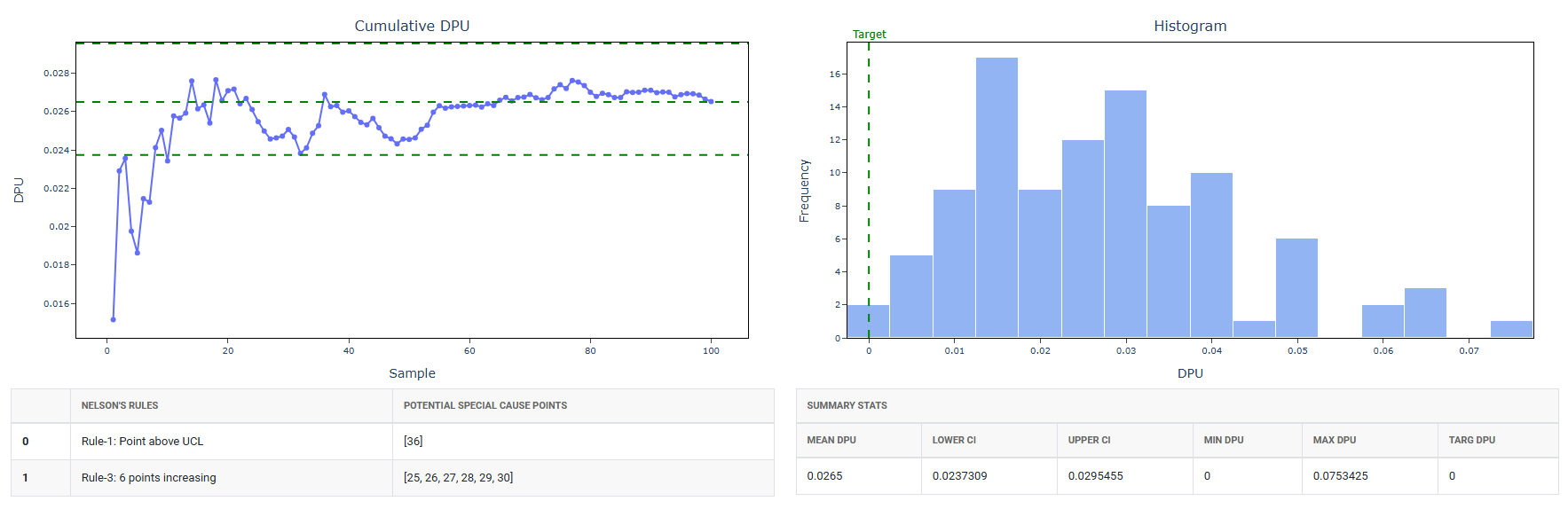
- The key output metrics are DPU (Defects Per Unit), DPMO (Defects Per Million Opportunities), and the sigma level — interpret these relative to your quality target rather than traditional Cp/Cpk thresholds.
Alternatives: When not to use Poisson Capability
| Situation | Use Instead |
| Each item is simply pass or fail (not a count of defects) | Binomial Capability Analysis |
| Data is continuous measured values | Normal, Non-Normal, or Nonparametric Capability Analysis |
| Count data shows overdispersion (variance >> mean) | Negative Binomial or Poisson with overdispersion model |
| Defect rate is high (not a rare event process) | Review process stability before capability analysis |
| Opportunity size varies significantly between units | Use U chart-based analysis with variable opportunity sizes |
Example of Poisson Capability
A process engineer is evaluating the durability of an electrical wire's insulation. The engineer randomly selects sections of wire and subjects them to a voltage test to identify weak spots in the insulation that could lead to failure during use. For each section of wire, the engineer records both the number of weak spots detected (defects) and the length of the wire in meters. The goal is to perform Poisson capability analysis to assess the insulation process's performance in meeting durability standards, determining if it consistently maintains the required quality level across different wire lengths. The following steps:
- Gathered the necessary data.
- Now analyses the data with the help of https://qtools.zometric.com/or https://intelliqs.zometric.com/.
- To find Poisson Capability choose https://intelliqs.zometric.com/> Statistical module> Process Capability>Poisson Capability.
- Inside the tool, feeds the data along with other inputs as follows:
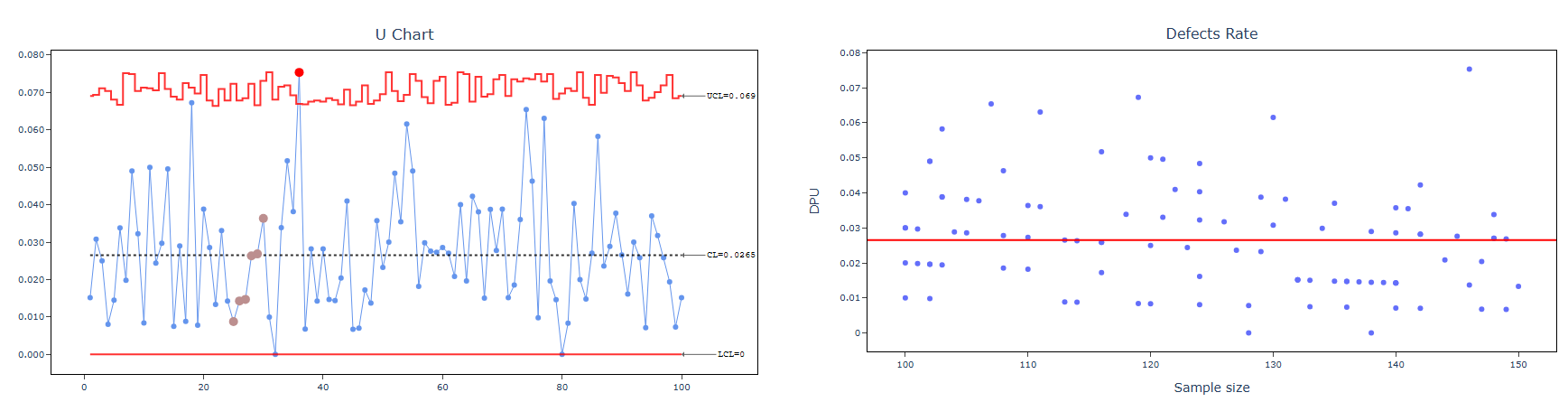
- After using the above mentioned tool, fetches the output as follows:
How to do Poisson Capability
The guide is as follows:
- Login in to QTools account with the help of https://qtools.zometric.com/ or https://intelliqs.zometric.com/
- On the home page, choose Statistical Tool> Process Capability >Poisson Capability .
- Next, update the data manually or can completely copy (Ctrl+C) the data from excel sheet and paste (Ctrl+V) it here.
- Fill the required options.
- Finally, click on calculate at the bottom of the page and you will get desired results.
On the dashboard of Poisson Capability, the window is separated into two parts.
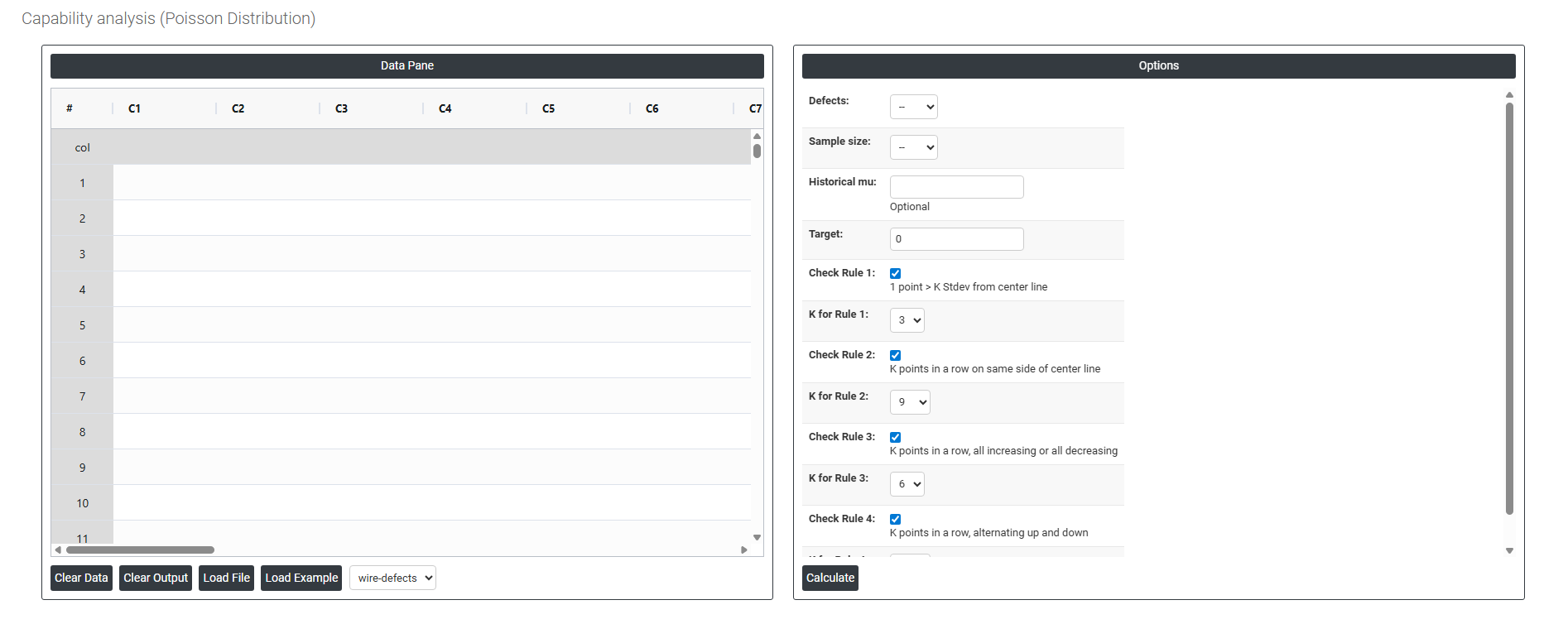
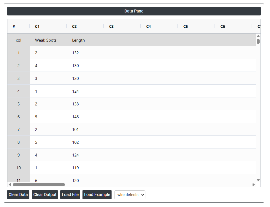
On the left part, Data Pane is present. In the Data Pane, each row makes one subgroup. Data can be fed manually or the one can completely copy (Ctrl+C) the data from excel sheet and paste (Ctrl+V) it here.
Load example: Sample data will be loaded.
Load File: It is used to directly load the excel data.
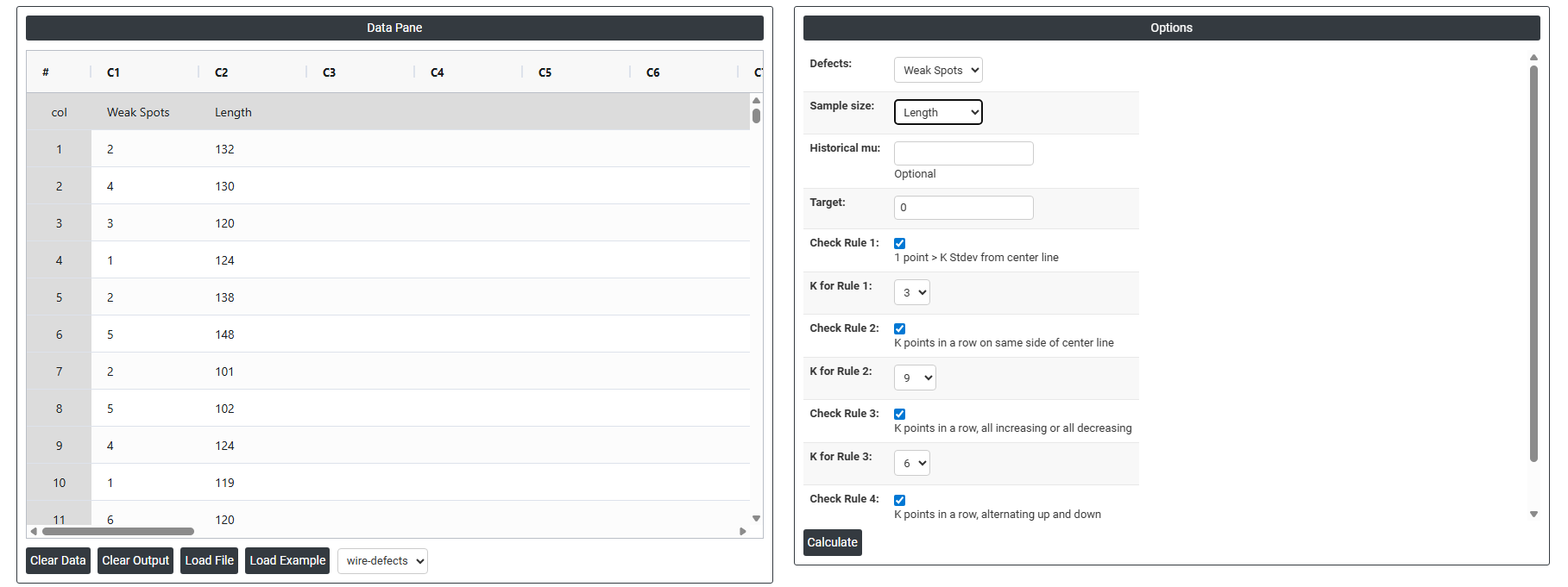
On the right part, there are many options present as follows:
- Defects Select the column containing the count of defects or occurrences recorded in each inspection period or subgroup for example, the number of surface scratches per panel, errors per document, or faults per unit length of cable. Each value in this column represents the total number of defects observed in one inspection unit or time period. This is the primary input the analysis uses to estimate the process defect rate.
- Sample Size Select the column containing the number of units or the size of the inspection area corresponding to each defect count. This is essential because the defect rate is calculated by dividing the defect count by the sample size for example, 12 defects across 300 units inspected gives a rate of 0.04 defects per unit. If the sample size is the same for every row, a constant value can be entered instead of a column.
- Historical Mu (μ) Optional. Mu (μ) represents the known or historically established average defect rate for the process. If you have a reliable baseline defect rate from a previous study or a long-term process record, enter it here. When provided, the analysis uses this value directly to calculate capability statistics and set performance benchmarks — rather than estimating the defect rate from the current dataset alone. This produces more stable and consistent results, especially when the current sample is small. Leave blank to let the analysis estimate mu from the data.
- Target The desired or ideal defect rate that the process should achieve. Entering a target allows the analysis to compare current process performance directly against a defined goal for example, a target of 0.01 defects per unit means no more than 1 defect per 100 units is acceptable. This value is used as a benchmark in the output and is displayed as a reference line on the capability chart, making it easy to see how far the current process is from the desired performance level.
- Check Rule 1: 1 point > K Stdev from center line: Test 1 is essential for identifying subgroups that significantly deviate from others, making it a universally recognized tool for detecting out-of-control situations. To increase sensitivity and detect smaller shifts in the process, Test 2 can be used in conjunction with Test 1, enhancing the effectiveness of control charts.
- Check Rule 2: K points in a row on same side of center line: Test 2 detects changes in process centering or variation. When monitoring for small shifts in the process, Test 2 can be used in conjunction with Test 1 to enhance the sensitivity of control charts.
- Check Rule 3: K points in a row, all increasing or all decreasing: Test 3 is designed to identify trends within a process. This test specifically looks for an extended sequence of consecutive data points that consistently increase or decrease in value, signaling a potential underlying trend in the process behavior.
- Check Rule 4: K points in a row, alternating up and down: Test 4 is designed to identify systematic variations within a process. Ideally, the pattern of variation in a process should be random. However, if a point fails Test 4, it may indicate that the variation is not random but instead follows a predictable pattern.
- Check Rule 5: K out of K + 1 points > 2 standard deviation from center line (same side): Test 5 detects small shifts in the process.
- Check Rule 6: K out of K + 1 points > 1 standard deviation from center line (same side):Test 6 detects small shifts in the process.
- Check Rule 7: K points in a row within 1 standard deviation of center line (either side):Test 7 identifies patterns of variation that may be incorrectly interpreted as evidence of good control. This test detects overly wide control limits, which are often a result of stratified data. Stratified data occur when there is a systematic source of variation within each subgroup, causing the control limits to appear broader than they should be.
- Check Rule 8: K points in a row > 1 standard deviation from center line (either side):Test 8 detects a mixture pattern. In a mixture pattern, the points tend to fall away from the center line and instead fall near the control limits.