Two Sample t Test(Summarized)

What is Two Sample t Test(Summarized)?

When to use Two Sample t test(Summarized)?

• Use when raw data is not available but you have the mean, standard deviation, and sample size for each group.
• Use when working from published reports, external supplier data, or historical summaries where individual observations were not recorded.
• Use when comparing two independent groups based on reported statistics rather than collected measurements.
• Use when you want to quickly validate or cross-check conclusions from aggregated data without needing to reconstruct the full dataset.

Guidelines for correct usage of Two sample t test(Summarized)

• Verify that the summary statistics entered are accurate and from a reliable source — errors in the inputs directly produce incorrect test conclusions.
• Ensure that the summary statistics represent independent, unrelated groups — the test assumes no relationship between the two samples.
• Confirm the sample sizes are sufficient — small samples with non-normal distributions may produce unreliable results even from correct summary inputs.
• Set alpha before running the test — the standard default is 0.05.
• Be cautious when summary statistics come from heavily skewed or non-normal populations — the t test assumes normality, which cannot be verified without the raw data.

Alternatives: When not to use Two sample t test(Summarized)

• If raw data is available, always use the standard Two Sample T Test instead — it provides additional diagnostics and assumption checks.
• If the two samples are paired or matched, use Paired T Test
• If comparing more than two groups, use One-Way ANOVA
• If the goal is to confirm equivalence rather than difference, use Two Sample Equivalence Test

Example of Two sample t test(Summarized)?

An economist collects data on the monthly energy cost for 25 families in the current year to determine if there has been a change from the previous year when the mean cost was $200. They perform a One sample t test to test if the current year's energy cost is significantly different from $200. The test in following steps:

1. Gathered the necessary data.
2.  Now analyses the data with the help of  https://qtools.zometric.com/ or https://intelliqs.zometric.com/.
3.  To find One sample t-test(Summarized) choose https://intelliqs.zometric.com/> Statistical module> Hypothesis Test> Two sample t-test(Summarized).
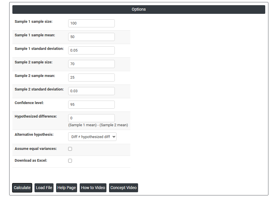
4.  Inside the tool, feeds the data along with other inputs as follows:

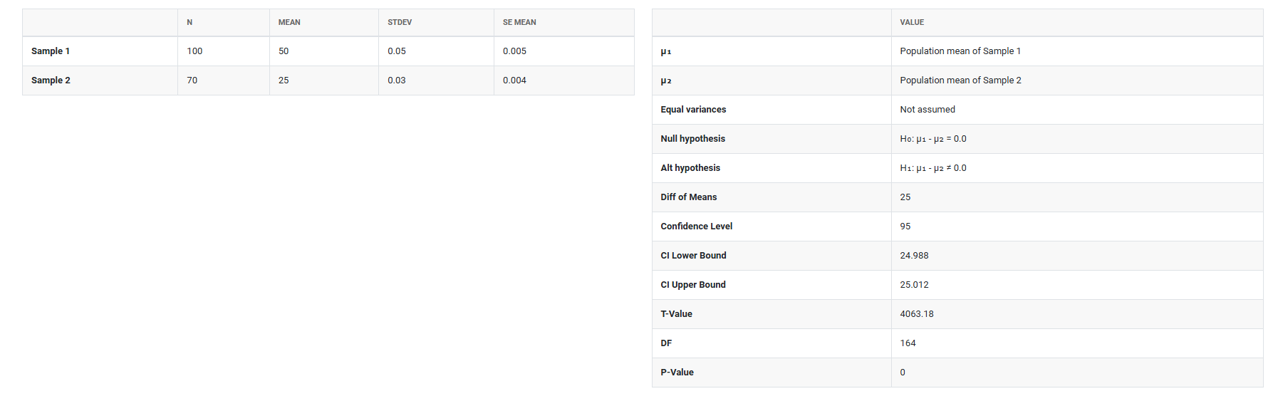
5. After using the above mentioned tool, fetches the output as follows:

How to do Two sample t test

The guide is as follows:

1. Login in to QTools account with the help of https://qtools.zometric.com/ or https://intelliqs.zometric.com/
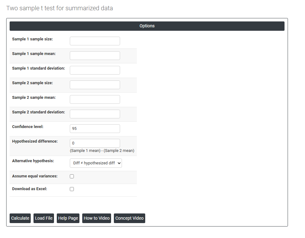
2. On the home page, choose Statistical Tool> Hypothesis Test >Two sample t test(Summarized) .
3. Next, update the data manually or can completely copy (Ctrl+C) the data from excel sheet and paste (Ctrl+V) it here.
4. Fill the required options..
5. Finally, click on calculate at the bottom of the page and you will get desired results.

On the dashboard of Two sample t test, the window is separated into two parts.

On the left part, Data Pane is present. In the Data Pane, each row makes one subgroup. Data can be fed manually or the one can completely copy (Ctrl+C) the data from excel sheet and paste (Ctrl+V) it here.

Load example: Sample data will be loaded.

Load File: It is used to directly load the excel data.

On the right part, there are many options present as follows:

• Sample 1 Sample Size: Enter the total number of observations in the first group — for example, if 40 measurements were taken from Formulation A, enter 40. This value is used to calculate the standard error and degrees of freedom for the test. A larger sample size produces more reliable and precise results.
• Sample 1 Sample Mean: Enter the average value of the first group's measurements. This is the central value around which the first group's data is distributed and is used directly in calculating the difference between the two groups.
• Sample 1 Standard Deviation: Enter the standard deviation of the first group — representing how much the individual measurements spread around the mean. A larger standard deviation indicates more variability within the group, which widens the confidence interval and reduces the test's sensitivity to detecting differences.
• Sample 2 Sample Size: Enter the total number of observations in the second group. Like Sample 1, this value contributes to the standard error calculation and influences how precisely the test can detect a real difference between the two groups.
• Sample 2 Sample Mean: Enter the average value of the second group's measurements. The test compares this directly against the Sample 1 mean to calculate the observed difference and determine whether it is statistically significant.
• Sample 2 Standard Deviation: Enter the standard deviation of the second group. This value reflects the spread of data in the second group and is used alongside the Sample 1 standard deviation to estimate the combined variability of the comparison.
• Confidence Level: Sets the certainty level for the confidence interval around the difference between the two means. The standard default is 95%, meaning you are 95% confident the true difference between the two population means falls within the displayed range. Increasing this to 99% widens the interval; reducing it to 90% narrows it.
• Hypothesized Difference: The assumed or expected difference between the two group means (Sample 1 mean minus Sample 2 mean) that you are testing against. Setting this to 0 tests whether the two means are equal. Setting it to any other value tests whether the actual difference equals that specific amount — for example, entering 10 tests whether Group 1 averages exactly 10 units more than Group 2.
• Alternative Hypothesis: Defines the direction of the test and what you are trying to prove about the difference. Three options are available:

• Diff ≠ Hypothesized Diff — a two-tailed test that checks whether the difference is simply not equal to the hypothesized value in either direction. Use when you have no prior expectation about which group will be larger.
• Diff < Hypothesized Diff — a one-tailed test that checks whether the actual difference is smaller than the hypothesized value. Use when you specifically expect Sample 1 to be lower than Sample 2.
• Diff > Hypothesized Diff — a one-tailed test that checks whether the actual difference is larger than the hypothesized value. Use when you specifically expect Sample 1 to be higher than Sample 2.

• Assume Equal Variances: When checked, the test assumes both groups share the same underlying population variance and uses a single pooled standard deviation for the calculation — producing a slightly more powerful test when the assumption is valid. When unchecked, separate variance estimates are used for each group (Welch's t test), which is more reliable when the two standard deviations entered are noticeably different. If uncertain, leave this unchecked as it is the safer and more conservative choice.
• Download as Excel: Exports the test results, summary statistics, confidence interval, and p-value into an Excel file for reporting, sharing, or record keeping.