What is Bootstrap 1-Sample ?
When to use Bootstrap 1-Sample?
- Use when the data does not meet normality assumptions and parametric confidence intervals may not be valid.
- Use when sample sizes are small and traditional methods based on normal approximations are unreliable.
- Use when estimating confidence intervals for statistics that have no simple analytical formula — such as the median, trimmed mean, or ratio of two quantities.
- Use to validate results from parametric tests by comparing bootstrap confidence intervals against traditionally calculated intervals.
Guidelines for correct usage of Bootstrap 1-Sample
- Use a sufficiently large number of bootstrap resamples — at least 1,000, and ideally 5,000 to 10,000 iterations, to ensure the bootstrap distribution is stable and reliable.
- Bootstrapping works best when the original sample is representative of the population — a biased or unrepresentative sample will produce biased bootstrap estimates.
- Do not use bootstrapping as a substitute for collecting adequate data — it cannot compensate for a poorly designed study or insufficient sample size.
- Results may vary slightly between runs due to random resampling — setting a random seed ensures reproducibility when reporting results.
Alternatives: When not to use Bootstrap 1-Sample
- If data is normally distributed and sample size is adequate, use standard parametric methods such as One Sample T Test instead — they are more efficient.
- If you need to compare two groups, use Two Sample T Test or Mann-Whitney Test
- If the primary concern is distribution fitting rather than interval estimation, use Individual Distribution Identification
Example of Bootstrap 1-Sample
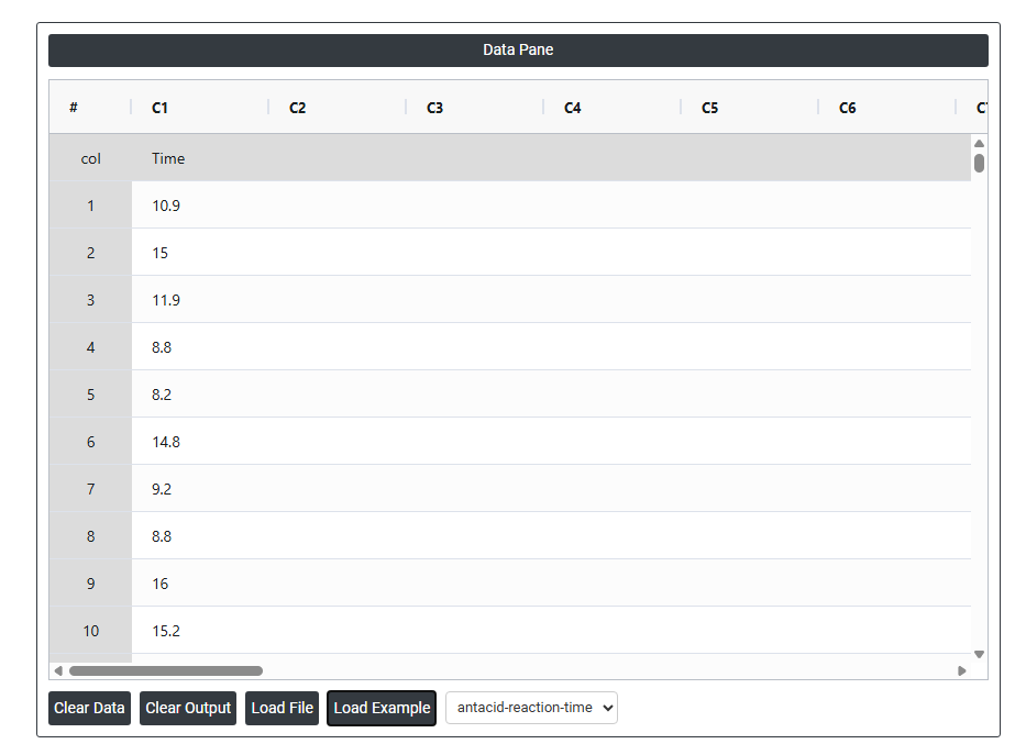
A chemist for a pharmaceutical company wants to determine the reaction time for a newly developed antacid. The test in following steps:
- Gathered the necessary data.
- Now analyses the data with the help of https://qtools.zometric.com/ or https://intelliqs.zometric.com/.
- To find Bootstrap 1-Sample choose https://intelliqs.zometric.com/> Statistical module> Hypothesis Test> Bootstrap 1-Sample.
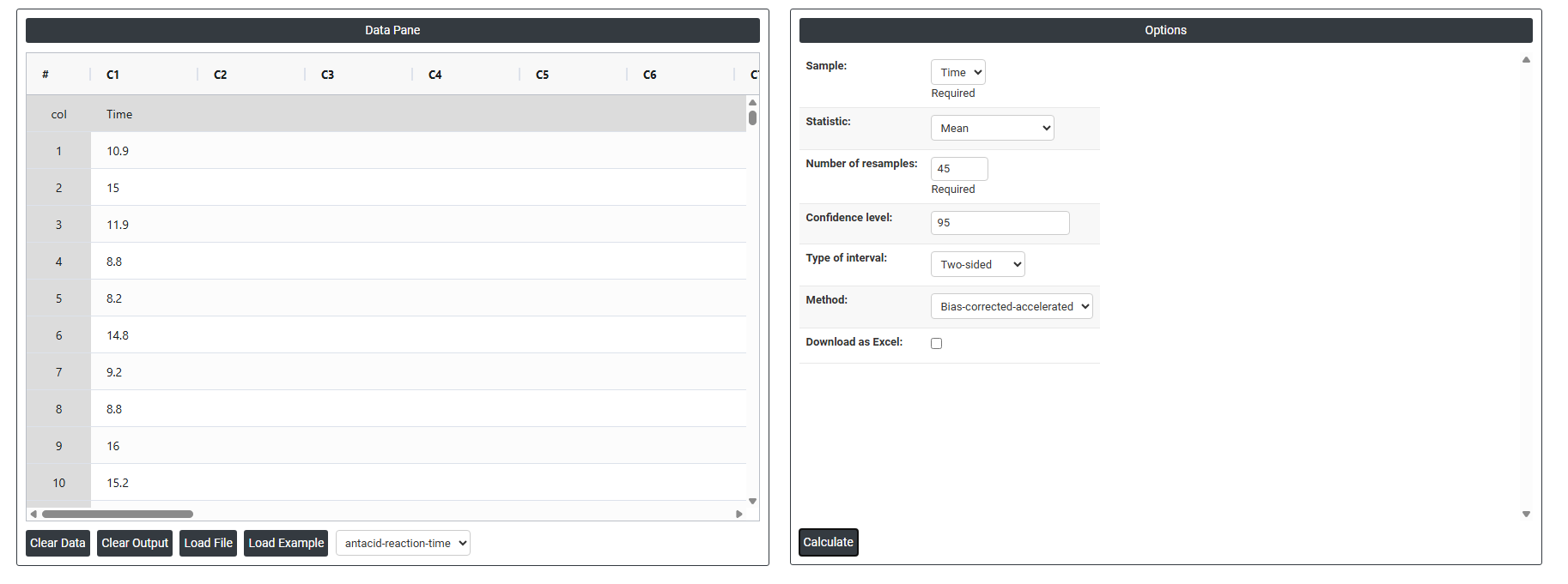
- Inside the tool, feeds the data along with other inputs as follows:
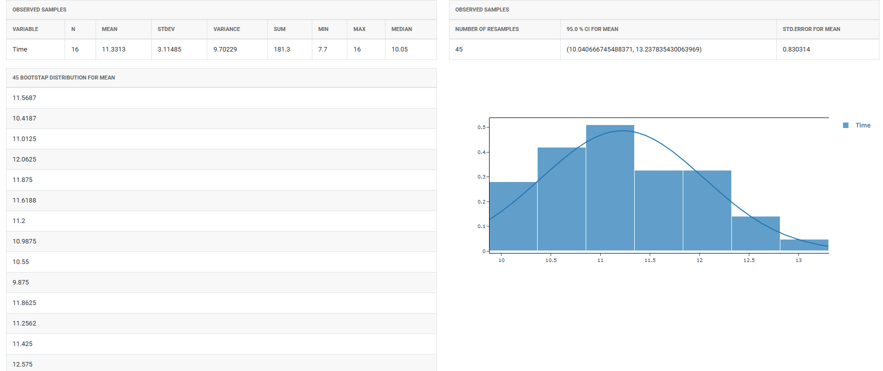
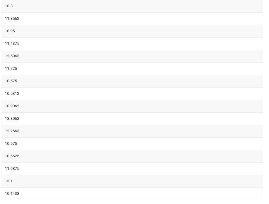
5. After using the above mentioned tool, fetches the output as follows:

How to do Bootstrap 1-Sample
The guide is as follows:
- Login in to QTools account with the help of https://qtools.zometric.com/ or https://intelliqs.zometric.com/
- On the home page, choose Statistical Tool> Hypothesis Test >Bootstrap 1-Sample .
- Next, update the data manually or can completely copy (Ctrl+C) the data from excel sheet and paste (Ctrl+V) it here.
- Fill the required options.
- Finally, click on calculate at the bottom of the page and you will get desired results.
On the dashboard of Bootstrap 1-Sample, the window is separated into two parts.
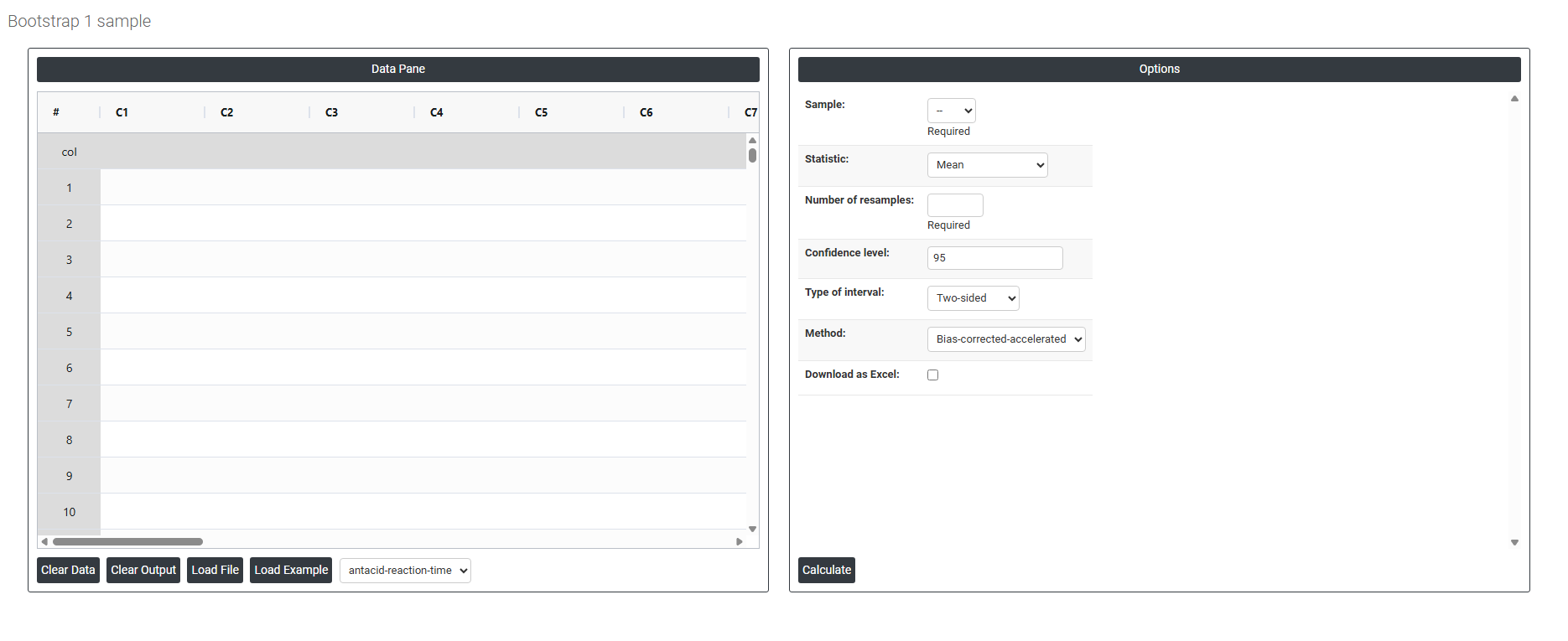
On the left part, Data Pane is present. In the Data Pane, each row makes one subgroup. Data can be fed manually or the one can completely copy (Ctrl+C) the data from excel sheet and paste (Ctrl+V) it here.
Load example: Sample data will be loaded.
Load File: It is used to directly load the excel data.
On the right part, there are many options present as follows:
- Sample: Select the column containing the raw data you want to analyse. This is the original dataset from which the bootstrap resamples will be drawn repeatedly with replacement. The quality and representativeness of this column directly determines the reliability of the bootstrap estimates — a biased or unrepresentative sample will produce biased bootstrap results. This field is required.
- Statistic: Select the statistical measure you want to estimate and build a confidence interval around. Six options are available:
- Mean — estimates the average value of the population and builds a confidence interval around it. The most commonly used option for general process analysis.
- Median — estimates the middle value of the population. More appropriate than the mean when data is skewed or contains outliers, as the median is less sensitive to extreme values.
- Sum — estimates the total sum of all values in the population. Useful when the cumulative total is the quantity of practical interest.
- Variance — estimates the spread of the population expressed as the squared standard deviation. Useful when understanding total variability is the primary goal.
- Standard Deviation — estimates the typical spread of individual values around the mean. More interpretable than variance as it is expressed in the original units of measurement.
- Number of Resamples: Enter the number of times the tool will randomly resample your data with replacement to build the bootstrap distribution. This field is required. A minimum of 1,000 resamples is recommended for basic analyses, and 5,000 to 10,000 is preferred for more precise and stable confidence interval estimates. More resamples produce smoother, more reliable results but require slightly more computation time.
- Confidence Level: Sets the certainty level for the bootstrap confidence interval. The standard default is 95%, meaning you are 95% confident that the true population statistic falls within the calculated interval. Increasing this to 99% produces a wider interval with greater certainty; reducing it to 90% produces a narrower interval with less certainty.
- Type of Interval: Defines the shape and direction of the confidence interval. Three options are available:
- Two-Sided — produces both a lower and upper bound, forming a complete interval around the statistic. Use when you are interested in how far the true value could be in either direction — this is the standard default for most analyses.
- Lower Bound — produces only a lower boundary, testing whether the true statistic is above a certain value. Use when only a minimum threshold matters — for example, confirming a process mean is at least a specified value.
- Upper Bound — produces only an upper boundary, testing whether the true statistic is below a certain value. Use when only a maximum threshold matters — for example, confirming that variability does not exceed an acceptable level.
- Method: Defines the mathematical approach used to calculate the bootstrap confidence interval from the resampled distribution. Four options are available:
- Bias-Corrected-Accelerated (BCa) — the most accurate and recommended method for most situations. It automatically adjusts for both bias (systematic error in the bootstrap estimate) and skewness in the bootstrap distribution, producing the most reliable confidence interval especially when the distribution of the statistic is not symmetric.
- Percentile — uses the direct percentiles of the bootstrap distribution to set the interval boundaries. Simple and intuitive but does not correct for bias or skewness — suitable when the bootstrap distribution is approximately symmetric and unbiased.
- Basic — also called the reflected percentile method, it reverses the percentile boundaries to correct for bias in a simple way. More reliable than the plain percentile method when the bootstrap distribution shows mild asymmetry.
- Download as Excel: Exports the normality test results, including the test statistic, p-value, and summary statistics, into an Excel file for reporting, sharing with colleagues, or maintaining a formal record of the analysis.