Try Statistical Software for Free
What is Johnson Transformation?
The Johnson Transformation is a statistical technique that converts non-normal data into a normal-like distribution, making it suitable for statistical analyses that require normality. It uses three distribution types—SU (unbounded), SB (bounded), and SL (lognormal)—to identify the best-fitting transformation based on data characteristics. Developed by Norman L. Johnson, this transformation is widely used in quality control and process capability studies. Statistical software typically automates the Johnson Transformation process, aiding in accurate interpretation of non-normal data.
When to use Johnson Transformation?
The Johnson Transformation is useful in the following :
- Non-Normal Data: When your data does not follow a normal distribution, especially if it has extreme skewness or kurtosis.
- Process Capability Analysis: For accurate capability indices (e.g., Cp, Cpk) in quality control, where normally distributed data is required.
- Control Charts: When non-normal data affects control chart accuracy, the transformation can improve chart sensitivity.
- Statistical Tests Requiring Normality: For tests like ANOVA or t-tests, which assume normality, the Johnson Transformation can help meet this assumption.
- Bounded Data: For data bounded on one or both sides, like percentages or counts, Johnson Transformation can normalize values effectively.
It’s commonly used in quality management, manufacturing, and Six Sigma projects.
Guidelines for correct usage of Johnson Transformation
- Data should be continuous, encompassing measurements that can assume any numeric value within a specified range along a continuous scale, including fractional and decimal values. Typical examples include variables such as length, weight, and temperature.
Alternatives: When not to use Johnson Transformation
- To perform normal capability analysis on non-normal data using a Johnson transformation without storing transformed values, you can directly select the Transform options within Normal Capability Analysis. For cases where a Box-Cox transformation is preferred—such as for control charts or in Individual Distribution Identification—this method is straightforward and intuitive but is limited to data with only positive values. Alternatively, if transforming the data is unnecessary, you can fit the data directly to a nonnormal distribution by using the Individual Distribution Identification option.
Example of Johnson Transformation
A quality engineer at a nutritional supplement company aims to evaluate the calcium content in vitamin capsules. The engineer gathers a random sample of capsules and measures their calcium levels. Based on previous observations, the engineer is aware that the data distribution is right-skewed.
To address this, the engineer applies the Johnson transformation to normalize the data and saves the transformed values in the worksheet for additional analysis. It performs the following steps:
- Gathered the necessary data.
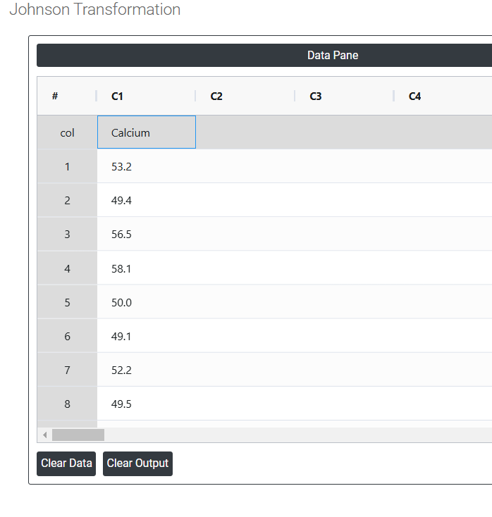
- Now analyses the data with the help of https://qtools.zometric.com/ or https://intelliqs.zometric.com/.
- To find Johnson Transformation choose https://intelliqs.zometric.com/> Statistical module> Control Charts>Johnson Transformation.
- Inside the tool, feeds the data along with other inputs as follows:
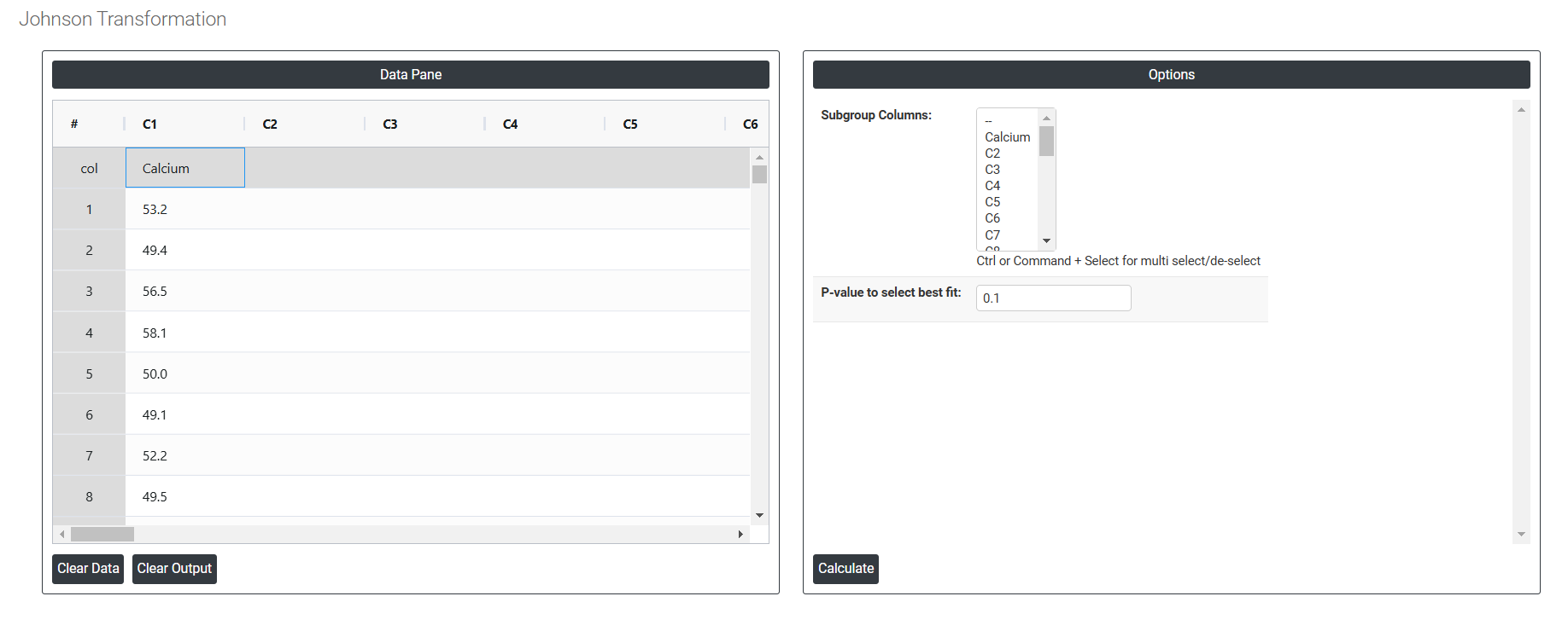
5. After using the above mentioned tool, fetches the output as follows:
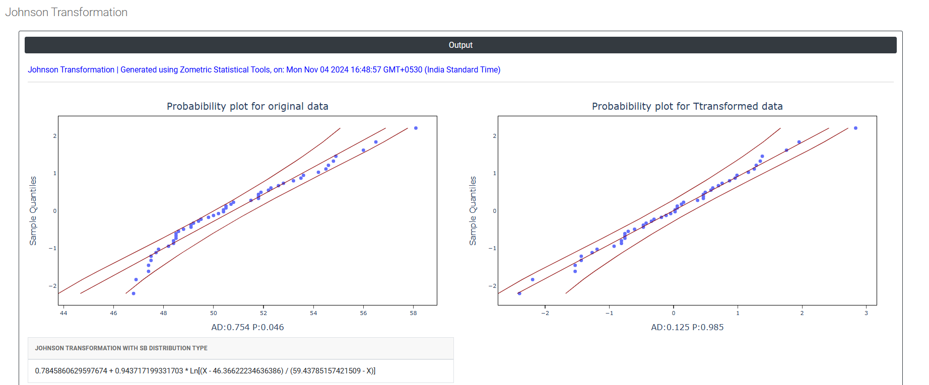
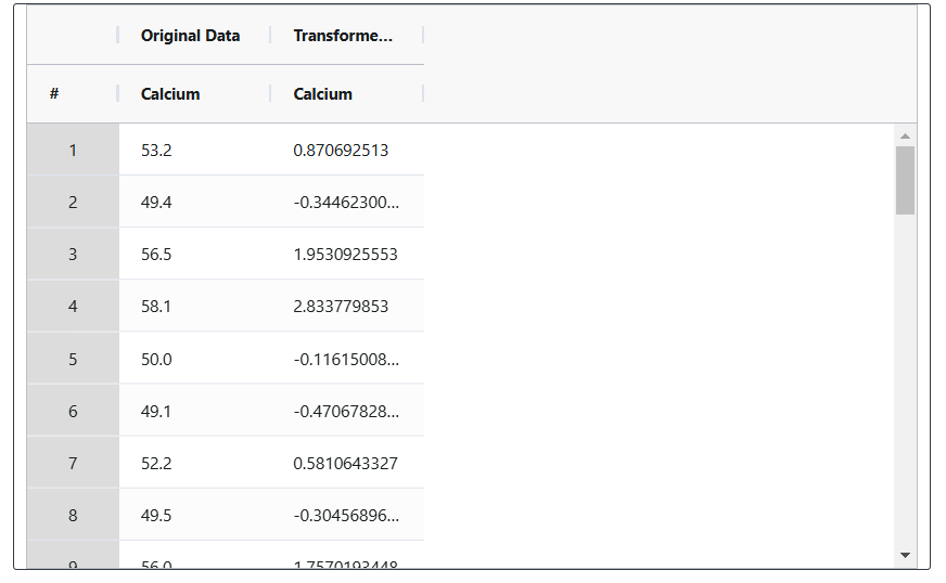
How to do Johnson Transformation
The guide is as follows:
- Login in to QTools account with the help of https://qtools.zometric.com/ or https://intelliqs.zometric.com/
- On the home page, choose Statistical Tool> Control Charts >Johnson Transformation.
- Click on Johnson Transformation and reach the dashboard.
- Next, update the data manually or can completely copy (Ctrl+C) the data from excel sheet and paste (Ctrl+V) it here.
- Next, you need to put the values of confidence level and hypothesized mean.
- Finally, click on calculate at the bottom of the page and you will get desired results.
On the dashboard of Johnson Transformation, the window is separated into two parts.
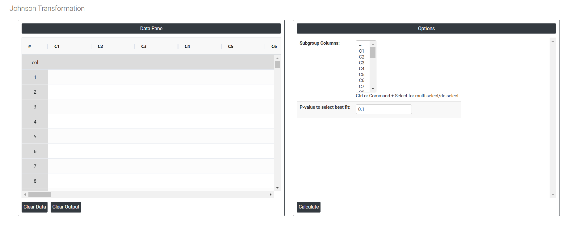
On the left part, Data Pane is present. In the Data Pane, each row makes one subgroup. Data can be fed manually or the one can completely copy (Ctrl+C) the data from excel sheet and paste (Ctrl+V) it here.
Load example: Sample data will be loaded.
Load File: It is used to directly load the excel data.
On the right part, there are many options present as follows:
- Subgroup Columns: Select the columns (Attribute name) according to the given data .
- P-value to select best fit: Input a value between 0 and 1 to set the significance level for testing data normality, both pre- and post-transformation. A higher significance level imposes stricter criteria for normality, while a lower value applies less stringent standards. To evaluate the distribution fit, an alpha level of 0.05 or 0.10 is often used.
- Download as Excel: This will display the result in an Excel format, which can be easily edited and reloaded for calculations using the load file option.