What is Binomial Capability?
Binomial Capability analysis measures how well a process performs when each inspected item results in one of exactly two outcomes typically classified as conforming or nonconforming, pass or fail, defective or non-defective. It evaluates the proportion of defective items the process produces and determines whether that proportion is low enough to meet a defined quality target or specification.
This type of capability analysis is built on the Binomial distribution, which mathematically models the probability of a fixed number of successes (or failures) in a series of independent trials. The primary performance metrics reported are the proportion defective, Parts Per Million (PPM) defective, and the equivalent sigma level giving a clear, standardized measure of how far the process is from zero defects.
Simple Definition: A capability analysis for pass/fail data it measures what proportion of your output is defective and tells you whether that rate meets your quality standard, expressed in PPM and sigma level.
When to use Binomial Capability?
- Use when each inspected item is classified into exactly two categories — such as pass/fail, good/bad, conforming/nonconforming, or present/absent.
- Use when you are monitoring the proportion or percentage of defective items produced by a process over time.
- Use when a fixed number of items are inspected in each subgroup, or when the subgroup size varies and is recorded separately.
- Use when each item's outcome is independent of all other items — the result of one inspection should not influence the next.
- Use when you have a defined maximum allowable proportion defective to benchmark performance against.
Guidelines for correct usage of Binomial Capability
- Confirm that each item is truly independently classified as defective or non-defective — items from the same batch or operator that are correlated will violate the Binomial assumption and inflate or deflate capability estimates.
- Ensure the process is stable and in statistical control before interpreting capability — use a P chart or Laney P' chart to verify stability first.
- Collect data from at least 25 subgroups to establish a reliable and stable estimate of the process proportion defective.
- The subgroup size should be large enough that each subgroup is likely to contain at least a few defective items — extremely small subgroups with a very low defect rate will produce unstable estimates.
- Key outputs include proportion defective, PPM defective, and the process sigma level — compare these against your quality target or customer requirement rather than traditional Cp/Cpk benchmarks.
- If overdispersion is detected (more variation than the Binomial model predicts), consider using Laney P' Chart for stability monitoring and acknowledge that the Binomial model may not perfectly describe the process.
Alternatives: When not to use Binomial Capability
| Situation | Use Instead |
| A single item can have multiple defects (not just pass/fail) | Poisson Capability Analysis |
| Data is continuous measured values | Normal, Non-Normal, or Nonparametric Capability Analysis |
| Response has more than two categories | Nominal or Ordinal Logistic analysis |
| Subgroup sizes are very small with near-zero defect rate | Collect larger subgroups before running capability analysis |
| Need to separate within and between variation sources | Capability Six Pack (Between/Within) |
Example of Binomial Capability
The supervisor for a call center wants to determine whether the call answering process is in control. The supervisor records the total number of incoming calls and the number of unanswered calls for 21 days. The following steps:
- Gathered the necessary data.
- Now analyses the data with the help of https://qtools.zometric.com/or https://intelliqs.zometric.com/.
- To find Binomial Capability choose https://intelliqs.zometric.com/> Statistical module> Process Capability>Binomial Capability.
- Inside the tool, feeds the data along with other inputs as follows:
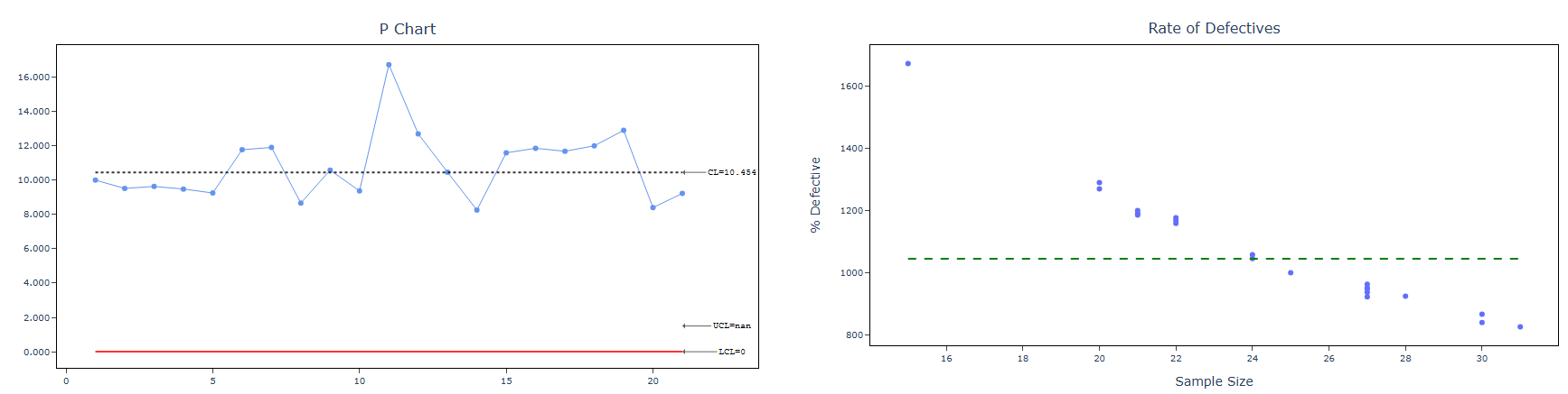
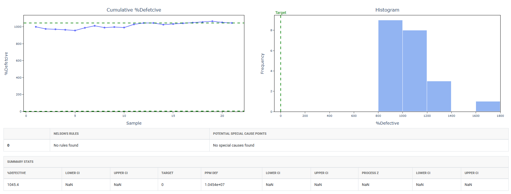
- After using the above mentioned tool, fetches the output as follows:
How to do Binomial Capability
The guide is as follows:
- Login in to QTools account with the help of https://qtools.zometric.com/ or https://intelliqs.zometric.com/
- On the home page, choose Statistical Tool> Process Capability >Binomial Capability .
- Next, update the data manually or can completely copy (Ctrl+C) the data from excel sheet and paste (Ctrl+V) it here.
- Fill the required options.
- Finally, click on calculate at the bottom of the page and you will get desired results.
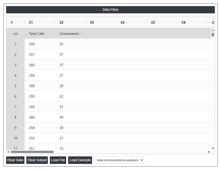
On the dashboard of Binomial Capability, the window is separated into two parts.
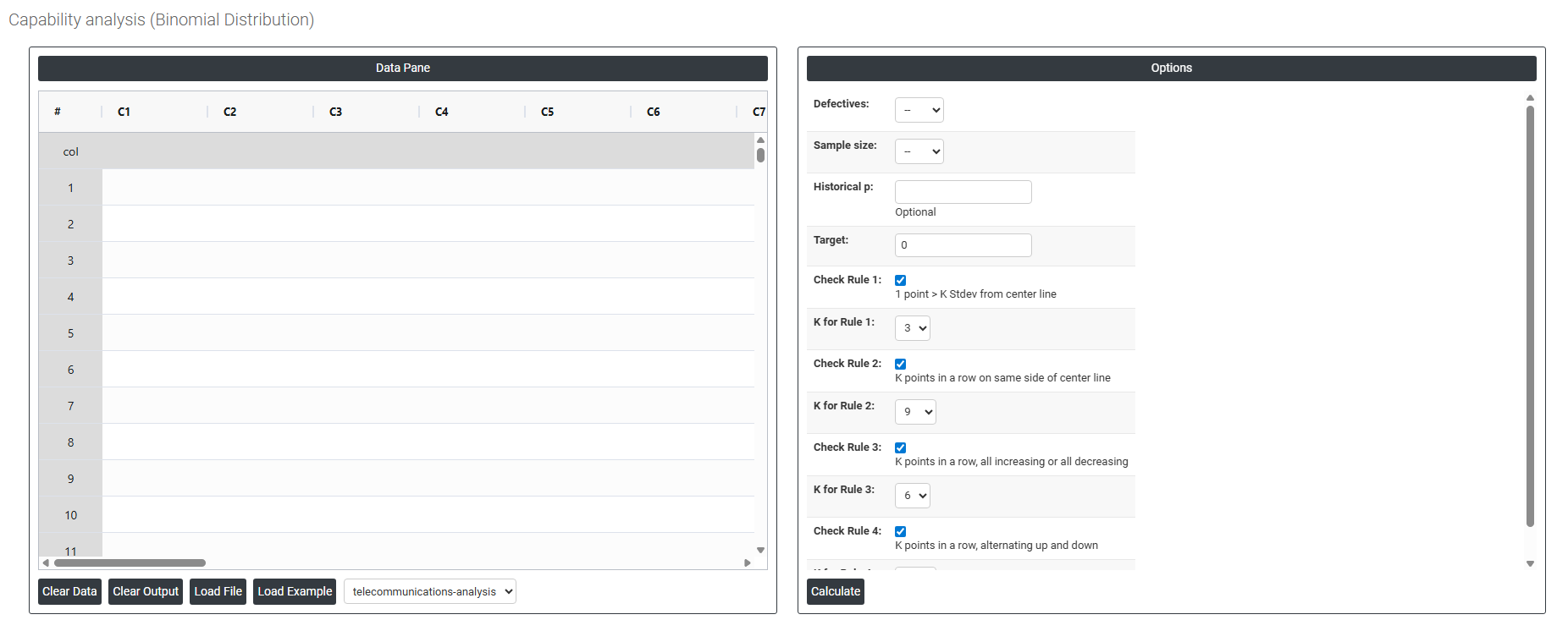
On the left part, Data Pane is present. In the Data Pane, each row makes one subgroup. Data can be fed manually or the one can completely copy (Ctrl+C) the data from excel sheet and paste (Ctrl+V) it here.
Load example: Sample data will be loaded.
Load File: It is used to directly load the excel data.
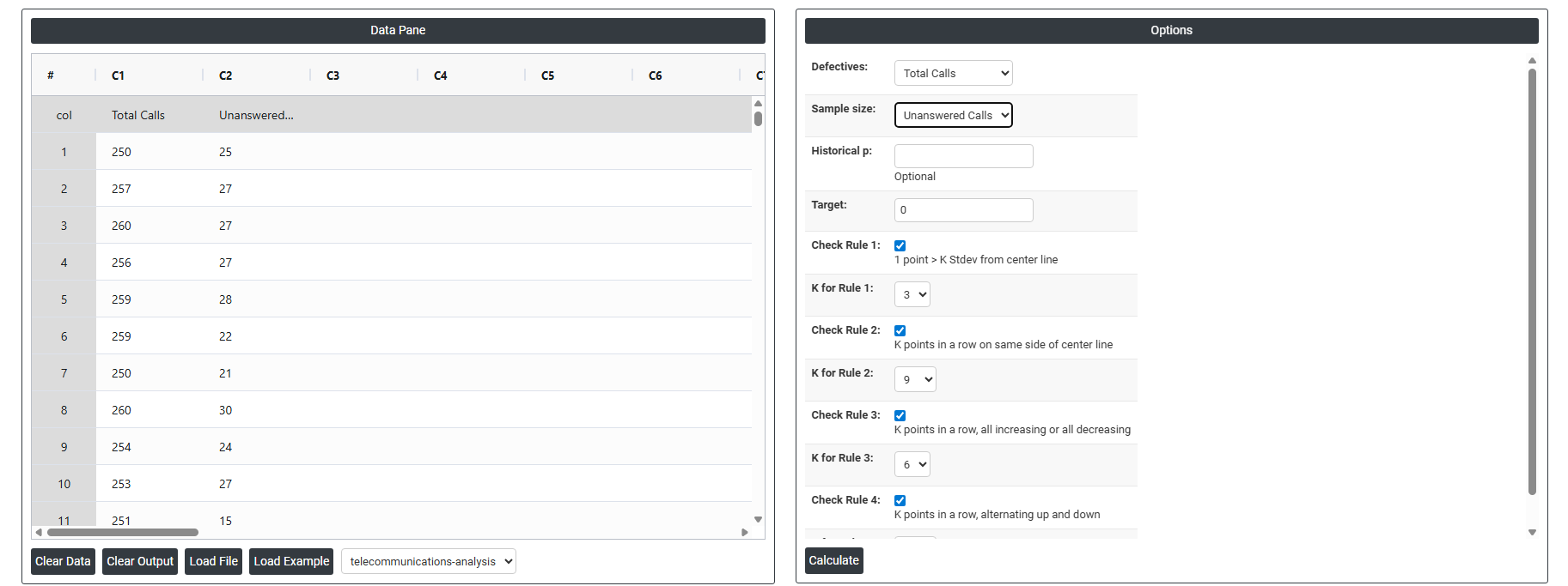
On the right part, there are many options present as follows:
- Defectives Select the column containing the count of defective items found in each subgroup or inspection period for example, the number of unanswered calls, rejected parts, or failed units recorded per time period. Each value in this column represents the total number of items classified as defective out of the total inspected. This is the primary input the analysis uses to estimate the proportion defective the process is producing.
- Sample Size Select the column containing the total number of items inspected in each subgroup or time period — for example, the total number of calls received, parts produced, or units examined per period. The proportion defective is calculated by dividing the defective count by the sample size for each subgroup. If the sample size is identical for every subgroup, a constant value can be entered directly instead of selecting a column.
- Historical p Optional. The letter p represents the known or historically established proportion defective for the process for example, 0.05 meaning 5% of items are typically defective. If a reliable baseline proportion has been determined from a previous long-term study or validated process record, enter it here. When provided, the analysis uses this value directly to calculate capability statistics and control limits rather than estimating it from the current data alone producing more stable, consistent results that reflect true long-term process performance. Leave blank to allow the analysis to estimate p from the current dataset.
- Target The desired or ideal proportion defective that the process should achieve — for example, entering 0.02 sets a target of no more than 2% defective items. When provided, this value is used as a performance benchmark in the output and displayed as a reference line on the capability chart, making it straightforward to see how far the current process performance is from the desired quality goal.
- Check Rule 1: 1 point > K Stdev from center line: Test 1 is essential for identifying subgroups that significantly deviate from others, making it a universally recognized tool for detecting out-of-control situations. To increase sensitivity and detect smaller shifts in the process, Test 2 can be used in conjunction with Test 1, enhancing the effectiveness of control charts.
- Check Rule 2: K points in a row on same side of center line: Test 2 detects changes in process centering or variation. When monitoring for small shifts in the process, Test 2 can be used in conjunction with Test 1 to enhance the sensitivity of control charts.
- Check Rule 3: K points in a row, all increasing or all decreasing: Test 3 is designed to identify trends within a process. This test specifically looks for an extended sequence of consecutive data points that consistently increase or decrease in value, signaling a potential underlying trend in the process behavior.
- Check Rule 4: K points in a row, alternating up and down: Test 4 is designed to identify systematic variations within a process. Ideally, the pattern of variation in a process should be random. However, if a point fails Test 4, it may indicate that the variation is not random but instead follows a predictable pattern.
- Check Rule 5: K out of K + 1 points > 2 standard deviation from center line (same side): Test 5 detects small shifts in the process.
- Check Rule 6: K out of K + 1 points > 1 standard deviation from center line (same side):Test 6 detects small shifts in the process.
- Check Rule 7: K points in a row within 1 standard deviation of center line (either side):Test 7 identifies patterns of variation that may be incorrectly interpreted as evidence of good control. This test detects overly wide control limits, which are often a result of stratified data. Stratified data occur when there is a systematic source of variation within each subgroup, causing the control limits to appear broader than they should be.
- Check Rule 8: K points in a row > 1 standard deviation from center line (either side):Test 8 detects a mixture pattern. In a mixture pattern, the points tend to fall away from the center line and instead fall near the control limits.