Create & Analyse Mixture DoE -

What is Create Mixture DoE?

Create Mixture DoE generates an experimental design for situations where the factors being studied are ingredient proportions that must add up to a fixed constant typically 100% or 1.0. In a mixture experiment, it is impossible to change one ingredient independently of the others because every increase in one ingredient requires a corresponding decrease in at least one other to maintain the fixed total.

Standard factorial designs cannot handle this constraint. Mixture designs use specialized design structures Simplex Lattice, Simplex Centroid, or Extreme Vertices that correctly explore the feasible ingredient space and produce design points that respect the mixture constraint at every run.

Simple Definitions: The design planning step for recipe and formulation experiments — generating a structured set of ingredient combinations that always sum to the required total, so you can discover the ideal blend that optimises product performance.

When to use Create Mixture DoE ?

Use when factors represent ingredient proportions that must sum to a fixed constant such as a paint formulation, food recipe, pharmaceutical compound, or chemical blend.
Use when you want to understand how changing relative proportions of ingredients affects product quality, performance, or properties.
Use when ingredients have upper and lower bound constraints for example, one component must comprise at least 15% but no more than 50% of the blend.
Use when process variables such as mixing speed or temperature also influence the response alongside the mixture components.

Guidelines for correct usage of Create Mixture DoE

Ensure all ingredient proportions sum exactly to the defined total at every experimental run deviations from the constraint will produce invalid data.
Set realistic upper and lower bounds for each ingredient before choosing the design type infeasible or overly tight constraints can produce an empty or impractical experimental space.
Use Extreme Vertices when ingredient constraints are present and Simplex Lattice or Centroid only when the full unconstrained space is accessible.
Prepare blends as accurately as possible small errors in ingredient proportions compound across runs and reduce the reliability of the model.
Randomise the order of blend preparation and testing to prevent systematic bias from measurement sequence, equipment drift, or analyst effects.

Alternatives: When not to use Create Mixture DoE

If factors are independent process variables rather than proportions summing to a constant, use Create Factorial DoE or Create Definitive Screening Design
If factors include both mixture components and process variables but you want to analyse them separately, design the mixture and process components independently first before combining.

What is Analyse Mixture DoE?

Analyse Mixture DoE fits a specialised mixture regression model called a Scheffé polynomial to the response data collected from a mixture experiment. Unlike standard regression, mixture models correctly account for the constraint that all ingredient proportions must sum to a constant, and they estimate how individual ingredients and their pairwise or higher-order blending combinations influence the response.

The analysis identifies which ingredients and blending interactions are significant, produces contour plots and trace plots to visualise the response surface across the mixture space, and generates the fitted model needed to run the Response Optimizer for finding the ideal blend.

When to use Analyse Mixture DoE ?

Use after completing a mixture design experiment and recording all response measurements from the prepared blends.
Use to identify which ingredients and ingredient combinations significantly influence the response.
Use to visualise the response surface across the mixture space using contour plots showing where in the blend space the best and worst responses are located.
Use to build the predictive model that will feed into Response Optimizer for finding the optimal blend formulation.

Guidelines for correct usage of Analyse Mixture DoE

Start with the simplest model that is scientifically reasonable Linear first, then Quadratic if blending effects are expected, then Special Cubic only if strong three-component synergies are suspected.
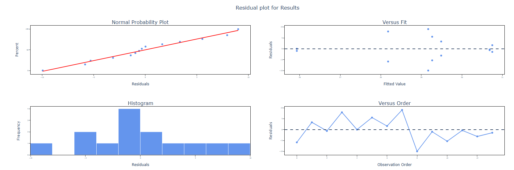
Check residual plots thoroughly before interpreting any results a model with non-random residuals should not be used to optimise blend formulations.
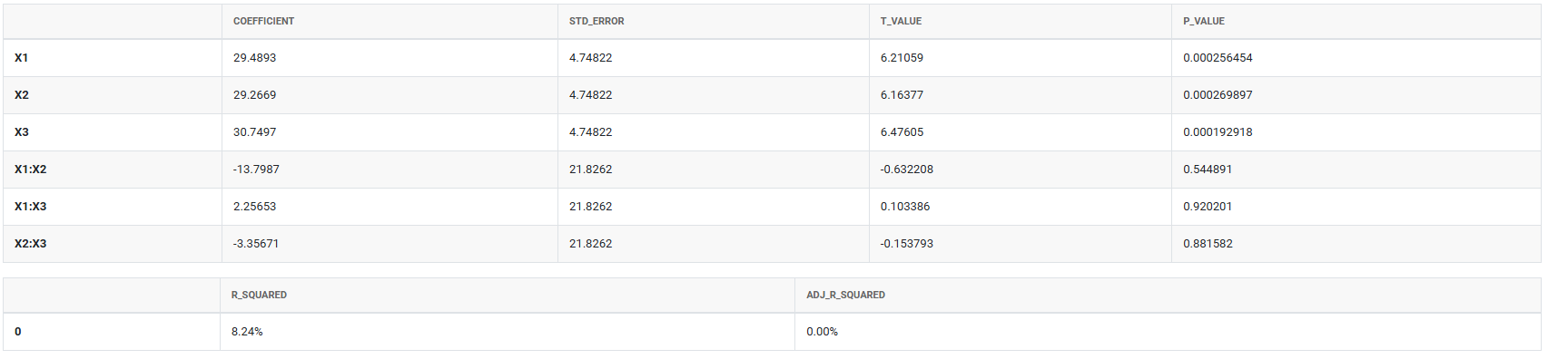
Use R-squared and adjusted R-squared to assess model fit a good mixture model typically achieves R-squared above 0.80 for a meaningful response.
Validate the best blend identified by the model with independent confirmation blends before moving to production — always verify predictions experimentally.
When process variables are included, check both the mixture terms and process variable terms for significance and do not simplify one at the expense of the other.

Alternatives: When not to use Analyse Mixture DoE

If the data came from a standard factorial experiment rather than a mixture design, use Analyse Factorial DoE instead Scheffé models are not appropriate for unconstrained factorial data.
If the response is binary or categorical, use a logistic regression approach rather than a standard mixture model.

Example of Create & Analyse Mixture DoE

The following steps:

Input the necessary data on right side panel Design & Analysis Inputs .

2. Now analyses the data with the help of https://qtools.zometric.com/ or https://intelliqs.zometric.com/.

3. To find Create & Analyse Mixture DoE choose https://intelliqs.zometric.com/> Statistical module> DOE>Create & Analyse Mixture DoE.

4. Click on Step 1. In the left-side panel under Designed Experiments & Results, the mixture design matrix will be generated. Add the response (outcome) variables as new columns at the end of the mixture design matrix.

5. In the right-side panel under Design & Analysis Inputs, locate the Responses option. Select the newly added outcome variable columns to define them as response variables.

6. Select the required interaction terms based on the experimental requirements

7. Click on Step 2 to perform the analysis of the designed experiment.

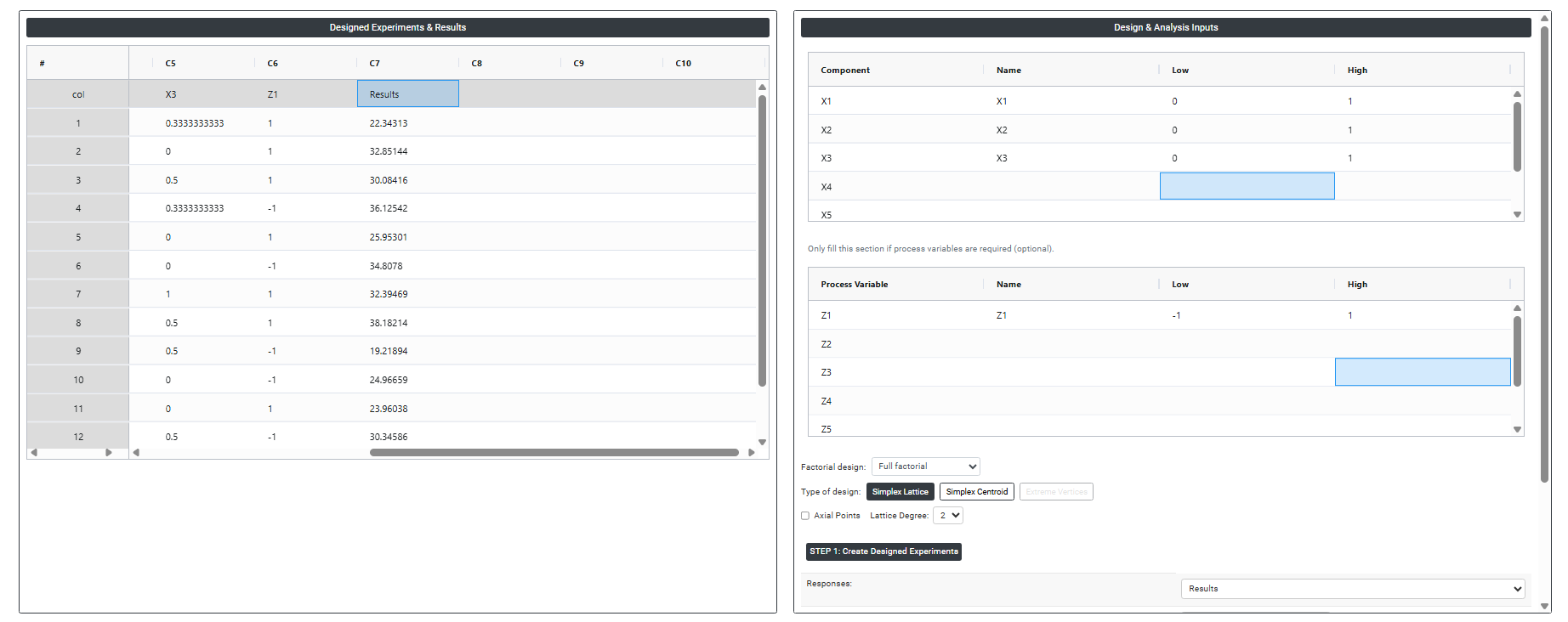
8. After using the above mentioned tool, fetches the output as follows:

How to do Create & Analyse Mixture DoE

The guide is as follows:

Login in to QTools account with the help of https://qtools.zometric.com/ or https://intelliqs.zometric.com/
On the home page, choose Statistical Tool> DOE>Create & Analyse Mixture DoE.
Next, update the data manually or can completely copy (Ctrl+C) the data from excel sheet or paste (Ctrl+V) .
Next, you need to fill the required options.
Click on Step 1. In the left-side panel under Designed Experiments & Results, the mixture design matrix will be generated. Add the response (outcome) variables as new columns at the end of the mixture design matrix.
In the right-side panel under Design & Analysis Inputs, locate the Responses option. Select the newly added outcome variable columns to define them as response variables.
Select the required interaction terms based on the experimental requirements
Click on Step 2 to perform the analysis of the designed experiment.

On the dashboard of Create & Analyse Mixture DoE, the window is separated into two parts.

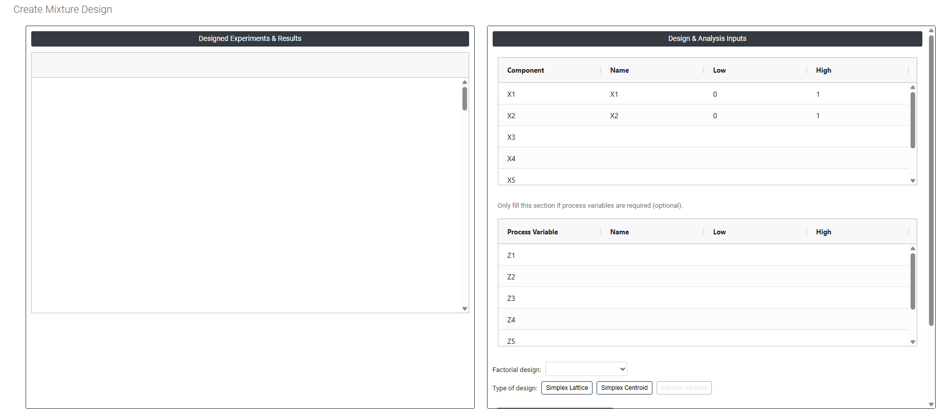
On the left part, Designed Experiments & Results is present. In the Designed Experiments & Results, it generates the design experiment.

On the right part, there are many options present as follows:

Component Variable Table: This is where you define each ingredient in your mixture. Every row represents one component of the blend, and each column captures a specific property of that ingredient.
- Name: The label you assign to each ingredient such as Water, Resin, Hardener, or Pigment. Use a clear, descriptive name so the design worksheet and output charts are easy to read and interpret.
- Low / High: The minimum and maximum levels at which this variable will be tested (default is 0 and 1 for coded values)
  - Sum of lower bounds must be less than 1.0 — If the minimum required amount of all ingredients combined already exceeds 100%, no valid blend exists and the design cannot be generated. For example, if you have three ingredients each with a lower bound of 0.40, the minimums alone sum to 1.20 which is impossible.
  - Sum of upper bounds must be greater than 1.0 — If the maximum allowed amount of all ingredients combined is less than 100%, again no valid blend can be constructed. For example, if three ingredients each have an upper bound of 0.30, the maximums sum to only 0.90 meaning it is impossible to fill the remaining 0.10.

Process Variable Table (Optional): If the experiment includes independent process conditions such as mixing time, processing temperature, or curing pressure in addition to the mixture components, define those variables here. The tool will combine the mixture design with a factorial structure for the process variables, creating a combined mixture-process design that estimates both ingredient blending effects and process effects simultaneously. This section only needs to be filled if your experiment includes independent process conditions alongside the mixture ingredients such as mixing speed, temperature, curing time, or pressure. Each process variable requires three inputs:
- Name — a meaningful label for the variable (e.g. Temperature, Speed)
- Low / High — the minimum and maximum levels at which this variable will be tested (default is −1 and +1 for coded values)
If your experiment involves only ingredient proportions and no process conditions, leave this section completely empty and proceed directly to the design type selection below.

Factorial Design: When process variables are added, this dropdown controls the fraction of all possible process variable combinations that will actually be tested. The available options depend entirely on how many process variables you have entered the tool automatically updates the dropdown to show only the fractions that are statistically valid for your variable count.

Here is exactly how the options appear based on the number of process variables entered:

Process Variables Entered	Available Factorial Design Options
1 variable	Full factorial only
2 variables	Full factorial only
3 variables	Full factorial, Half factorial
4 variables	Full factorial, Half factorial
5 variables	Full factorial, Half factorial, Quarter factorial
6 variables	Full factorial, Half factorial, Quarter factorial, Eighth factorial
7 variables	Full factorial, Half factorial, Quarter factorial, Eighth factorial, Sixteenth factorial

Why does this happen?

Fractional factorial designs only make statistical sense when there are enough variables to justify splitting. With 1 or 2 process variables, a full factorial is only 2 or 4 runs there is nothing to meaningfully fractionate. As the variable count grows, more fractions become available because there are enough factor combinations to split without losing important information.

What Each Factorial Design Option Means

Full Factorial: Tests every possible combination of process variable levels. If you have 3 process variables each at 2 levels, this is 8 runs. Provides complete information about all main effects and interactions. Always available regardless of how many variables you have.
Half Factorial: Tests half of all possible combinations (fraction = 1/2). Reduces runs by 50% compared to full factorial. Some two-factor interactions become confounded with main effects. Available from 3 variables onwards.
Quarter Factorial: Tests one quarter of all possible combinations (fraction = 1/4). Reduces runs by 75%. More confounding occurs but main effects remain estimable. Available from 5 variables onwards.
Eighth Factorial: Tests one eighth of all possible combinations (fraction = 1/8). Very compact primarily useful for initial screening when many process variables are present and run count must be kept minimal. Available from 6 variables onwards.
Sixteenth Factorial: Tests one sixteenth of all possible combinations (fraction = 1/16). The most extreme reduction available. Only main effects can typically be estimated cleanly interactions are heavily confounded. Available only when 7 or more process variables are entered.

Type Of Designs:
- Simplex Lattice: Places design points at regularly spaced proportions across the mixture simplex including pure components, binary blends, ternary blends, and so on depending on the degree chosen. The higher the degree, the more design points are included and the more complex the blending model that can be fitted. Best suited for studying the full mixture space without ingredient constraints.
  - Lattice Degree: Controls how many proportion values each ingredient can take (from 0 to 1), determining design complexity and the model you can fit.

- - - Degree 2 — Values: 0, ½, 1. Fits a quadratic model. Best for initial studies where pairwise blending effects are the main interest.
    - Degree 3 — Values: 0, ⅓, ⅔, 1. Fits a special cubic model. Use when three-component interactions are suspected.
    - Degree 4 — Values: 0, ¼, ½, ¾, 1. Fits a quartic model. Only for confirmed highly non-linear blending rarely needed.

- - Axial Points: Sit midway between each component's pure vertex and the centroid, with one ingredient high and the rest shared equally.
    - Include when: using Degree 2 with 3–5 components, pure vertices aren't achievable, or you need better centroid-region predictions.
    - Exclude when: minimising runs, already on Degree 3/4, using 6+ components, or tight constraints make axial points infeasible (use Extreme Vertices instead).
- Simplex Centroid: Includes design points at the pure component vertices, at the midpoints of each binary blend, at the centroid of each ternary blend, and at the overall mixture centroid. This design provides good coverage across the entire mixture space and supports fitting of models that capture how pairs and groups of ingredients interact. Best used when no ingredient constraints are present.
  - Axial Points: Sit midway between each component's pure vertex and the centroid, with one ingredient high and the rest shared equally.
    - Include when: Using Degree 2 with 3–5 components, pure vertices aren't achievable, or you need better centroid-region predictions.
    - Exclude when: Minimizing runs, already on Degree 3/4, using 6+ components, or tight constraints make axial points infeasible (use Extreme Vertices instead).
- Extreme Vertices: Used when one or more ingredients have upper or lower bound constraints that restrict the feasible mixture region to a sub-space of the full simplex. The design points are placed at the corners (vertices), edge midpoints, and centroid of this constrained feasible region ensuring the experiment explores only practically achievable blends. This is the correct choice when ingredient constraints are present.
- Responses: Enter the name and unit for each output variable to be measured from the prepared blends such as viscosity, hardness, yield, or shelf life. Multiple responses can be recorded from the same set of experimental blends, enabling simultaneous optimization of several product properties from a single experiment.
- Select Terms: Choose which mixture model terms to include in the eventual analysis. Common choices include Linear (first-order blending), Quadratic (pairwise blend interactions). Start with the simplest model that is scientifically reasonable and expand only if the data supports it.

Try Statistical Software for Free