What is CUSUM Chart?
A CUSUM Chart (Cumulative Sum Chart) detects small but sustained shifts in the process mean by accumulating the deviations of each measurement from the target value over time. Instead of plotting each data point individually, it tracks the running total of how far measurements have drifted above or below the target — making even tiny, consistent shifts visible long before a standard control chart would flag them.
The cumulative sum builds up gradually when the process shifts away from target. If it grows large enough to cross a decision boundary (called the H value or decision interval), a signal is generated. This sensitivity to small sustained shifts is what makes CUSUM charts uniquely powerful compared to standard Shewhart charts like I-MR or Xbar-R.
When to use CUSUM Chart?
- Use when you need to detect small, sustained shifts in the process mean — typically shifts of 0.5 to 2 standard deviations that a standard chart would miss.
- Use when the cost of missing a small process drift is high — such as in pharmaceutical manufacturing, precision engineering, or food safety processes.
- Use with individual continuous measurements or subgroup means collected in time order.
- Use when a target value is known or specified — the CUSUM chart works by measuring deviations from this target, so a meaningful target is essential.
Guidelines for correct usage of CUSUM Chart
- Set the reference value (K) to half the size of the shift you want to detect — for example, if detecting a 1-sigma shift, set K to 0.5.
- Set the decision interval (H) — a value of 4 to 5 standard deviations is the common standard, balancing sensitivity against false alarm rate.
- Data must be collected in strict time order — the cumulative sum loses meaning if observations are out of sequence.
- Data should be approximately normally distributed for the statistical properties of the CUSUM chart to hold.
- Once a signal occurs, reset the CUSUM to zero after investigating and resolving the root cause before continuing to monitor.
- Collect at least 20 baseline observations to estimate the process mean and standard deviation before running the CUSUM chart.
Alternatives: When not to use CUSUM Chart
- If you need to detect large, sudden process shifts, use I-MR Chart or Xbar-R Chart instead — Shewhart charts react faster to abrupt changes.
- If no meaningful target value exists for your process, the CUSUM chart cannot be properly set up — use I-MR or Moving Average Chart
- If the data is attribute-based (counts or proportions), use appropriate CUSUM variants for attribute data or switch to P, NP, C, or U charts.
- If you want a simpler chart with similar small-shift sensitivity, use EWMA Chart instead — it is easier to set up and interpret for most users.
Example of CUSUM Chart?
A quality engineer at an automobile engine assembly plant observes the vertical displacement of crankshafts during engine operation. To track this movement, the engineer recorded measurements with a subgroup size of 1 The following steps:
- Gathered the necessary data.
- Now analyses the data with the help of https://qtools.zometric.com/ or https://intelliqs.zometric.com/.
- To find CUSUM Chart choose https://intelliqs.zometric.com/> Statistical module> Control Chart > CUSUM Chart.
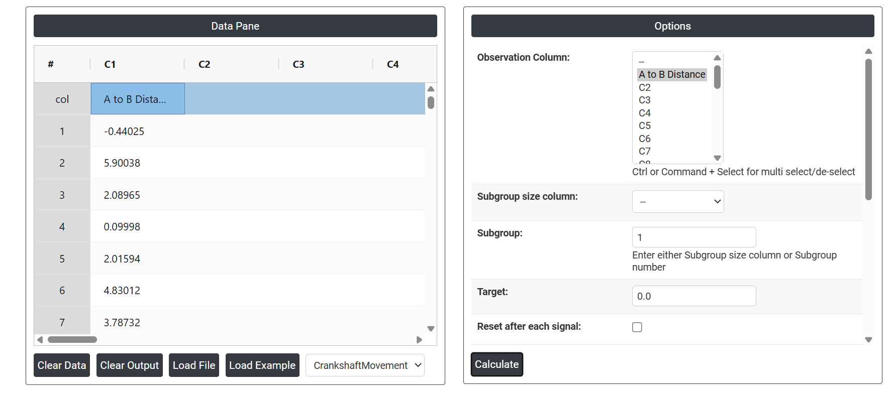
- Inside the tool, feed the data along with other inputs as follows:
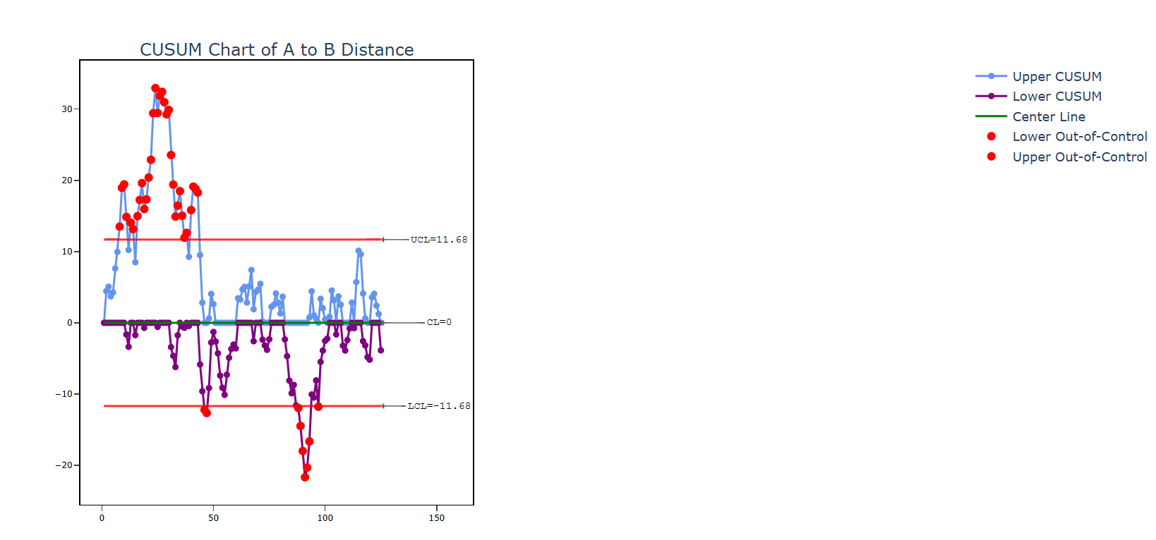
5. After using the above-mentioned tool, fetches the output as follows:
How to generate CUSUM Chart?
The guide is as follows:
- Login in to QTools account with the help of https://qtools.zometric.com/ or https://intelliqs.zometric.com/
- On the home page, choose Statistical Tool> Control Chart > CUSUM Chart.
- Next, update the data manually or can completely copy (Ctrl+C) the data from excel sheet or paste (Ctrl+V) it or else there is say option Load Example where the example data will be loaded.
- Finally, click on calculate at the bottom of the page and you will get desired results.
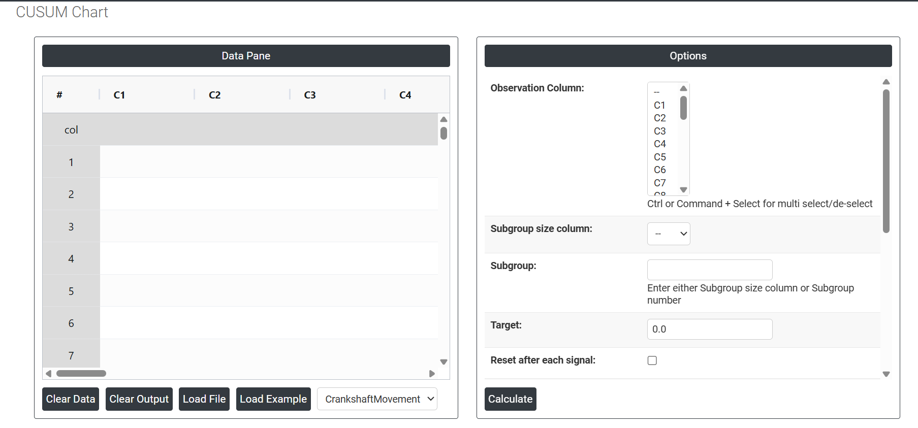
On the dashboard of CUSUM Chart the window is separated into two parts.
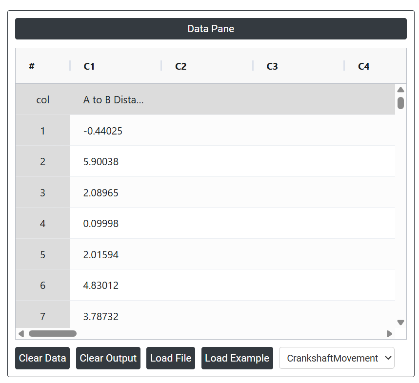
On the left part, Data Pane is present. In the Data Pane, each row makes one subgroup. Data can be fed manually or the one can completely copy (Ctrl+C) the data from excel sheet and paste (Ctrl+V) it here.
Load example: The sample data will be loaded.
Load File: It is used to directly load the excel data.
On the right part, there are many options present as follows:
- Observation Column Select the column(s) containing your measurement data. Use Ctrl or Command + Click to select multiple columns. These are the individual or subgrouped values — such as dimensions, temperatures, or weights — that the chart will use to accumulate deviations from the target and detect sustained process shifts.
- Subgroup Size Column Select the column that identifies which observations belong to which subgroup when subgroup sizes vary across time periods. Either this field or the Subgroup Number must be provided — not both. Use this when the number of measurements per subgroup is not consistent throughout the dataset.
- Subgroup Enter a fixed number if all subgroups contain the same number of observations. When set to 1, the chart monitors individual measurements. When greater than 1, subgroup means are calculated first and then the cumulative sum is tracked across those means.
- Target The reference value from which all deviations are accumulated. This is the most critical input for a CUSUM chart — every measurement is compared to this target and the difference is added to the running sum. If no target is entered, the chart estimates it from the data. For best results, always enter a known process target or specification centre value rather than relying on estimation.
- Reset After Each Signal When enabled, the cumulative sum resets back to zero each time an out-of-control signal is detected. This prevents a past signal from continuing to influence the chart after a root cause has been identified and addressed. It is recommended to enable this option so that each new phase of monitoring starts fresh after a confirmed process change.
- h (Decision Interval) Sets the threshold boundary on the CUSUM chart. When the cumulative sum exceeds this value in either direction, a signal is generated indicating the process has shifted. The standard default is 4 or 5, expressed in standard deviation units. A smaller h makes the chart more sensitive and generates signals faster but increases the risk of false alarms. A larger h reduces false alarms but takes longer to detect real shifts.
- k (Reference Value / Allowable Slack) Defines the size of the shift you want the chart to be most sensitive to, expressed as a proportion of the standard deviation. Each new measurement is adjusted by k before being added to the cumulative sum — effectively filtering out small, acceptable random variation and only accumulating evidence of shifts larger than k. The standard default is 0.5, which optimises the chart to detect a shift of 1 standard deviation. Set k to half the shift size you most want to detect.
- Standard Deviation Optional. If you have a known or historically validated standard deviation for the process, enter it here. When provided, this value is used directly to scale the CUSUM calculations and set the decision boundaries instead of estimating spread from the current data — producing more accurate and stable signals when a reliable baseline exists.
- SD Estimation Method for Subgroup Size = 1 Controls how standard deviation is estimated when data consists of individual measurements. Two options are available:
- Average Moving Range — estimates standard deviation by averaging the moving ranges between consecutive observations. This is the standard default and works reliably for most individual measurement processes.
- Median Moving Range — uses the median of the moving ranges instead, making the estimate more robust against the influence of outliers or sudden unusual spikes in the data.
- SD Estimation Method for Subgroup Size > 1 Controls how standard deviation is estimated when data is collected in subgroups of two or more. Three options are available:
- Pooled Stdev — combines standard deviations from all subgroups into one pooled estimate, providing a stable and accurate overall measure of within-subgroup variation.
- Rbar — estimates standard deviation from the average of subgroup ranges. Simple and reliable for subgroup sizes of 2 to 8.
- Sbar — estimates standard deviation from the average of subgroup standard deviations. More accurate than Rbar for subgroup sizes greater than 8.
- Length Moving Range Defines how many consecutive observations are used to calculate each moving range value when estimating standard deviation. The default is 2, meaning each moving range is the absolute difference between two consecutive measurements. Increasing this value smooths the estimate but reduces sensitivity to short-term variation changes.
- Use Unbiasing Constant When checked, applies a statistical correction factor that removes the small mathematical bias naturally present when estimating standard deviation from sample data. This improves the precision of control limit and decision boundary calculations and is recommended to keep enabled for more accurate results.