What is Graphical Summary?
Graphical Summary is an all-in-one analysis tool that combines key numerical statistics with multiple visual representations of your data in a single, consolidated output. It typically displays a histogram, a boxplot, a confidence interval plot for the mean, and a normal probability plot — all presented together alongside descriptive statistics such as the mean, standard deviation, and normality test results.
By combining visuals and numbers in one view, Graphical Summary gives you a fast and complete understanding of your data — its shape, centre, spread, outliers, and normality — without needing to run multiple separate tools.
When to use Graphical Summary?
- Use as an early exploration step at the beginning of a study to quickly understand the structure and behaviour of a new dataset.
- Use when presenting data to a mixed technical and non-technical audience — the combined visual and numerical output is easy to read for everyone.
- Use when performing initial data quality checks — the histogram and boxplot immediately reveal outliers, gaps, or unusual patterns.
- Use when you want to verify normality visually and statistically in one step before proceeding to capability analysis or hypothesis testing.
Guidelines for correct usage of Graphical Summary
- Review the histogram shape first — a symmetric bell shape suggests normality; a skewed or multi-peaked histogram suggests otherwise.
- Check the boxplot for outliers — any points plotted beyond the whiskers are potential outliers that warrant investigation before further analysis.
- Use the Anderson-Darling p-value in the output to formally confirm or reject normality — a p-value above 0.05 generally supports normality.
- Collect at least 20 observations for the visual displays and normality test to give meaningful and stable results.
- Do not use Graphical Summary as a substitute for a formal hypothesis test — it is an exploratory and diagnostic tool, not a decision-making test in itself.
Alternatives: When not to use Graphical Summary
| Situation | Use Instead |
| Only need numerical summaries without visuals | Descriptive Statistics |
| Need to assess normality in detail only | Normal Probability Plot |
| Need to detect trends or shifts over time | Run Chart or Control Chart |
| Data is categorical (not continuous) | Bar Chart or Pie Chart |
Example of Graphical Summary
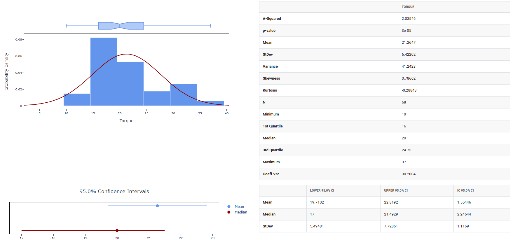
A quality control engineer needs to ensure that the caps on shampoo bottles are fastened correctly. If the caps are fastened too loosely, they may fall off during shipping. If they are fastened too tightly, they may be too difficult to remove. The target torque value for fastening the caps is 18. The engineer collects a random sample of 68 bottles and tests the amount of torque that is needed to remove the caps. The following steps:
- Gathered the necessary data.
- Now analyses the data with the help of https://qtools.zometric.com/ or https://intelliqs.zometric.com/.
- To find Graphical Summary choose https://intelliqs.zometric.com/> Statistical module> Graphical analysis > Graphical Summary.
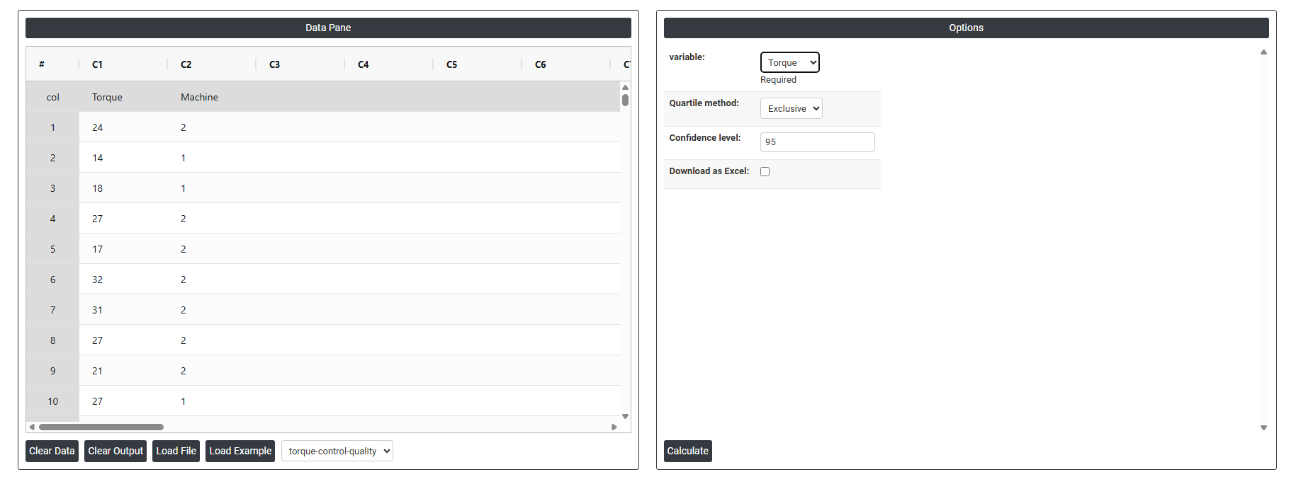
- Inside the tool, feed the data along with other inputs as follows:
6. After using the above-mentioned tool, fetches the output as follows:
How to do Graphical Summary
The guide is as follows:
- Login in to QTools account with the help of https://qtools.zometric.com/ or https://intelliqs.zometric.com/
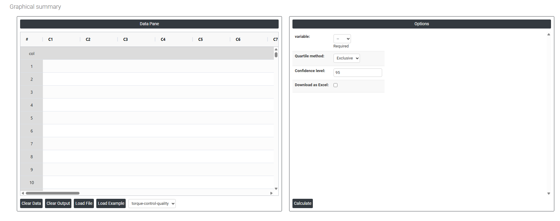
- On the home page, choose Statistical Tool> Graphical analysis > Graphical Summary.
- Next, update the data manually or can completely copy (Ctrl+C) the data from excel sheet or paste (Ctrl+V) it or else there is say option Load Example where the example data will be loaded.
- Next, you need to fill the required options.
- Finally, click on calculate at the bottom of the page and you will get desired results.
On the dashboard of Graphical Summary, the window is separated into two parts.
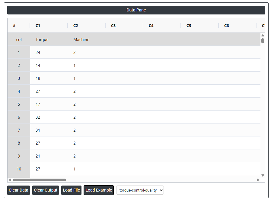
On the left part, Data Pane is present. In the Data Pane, each row makes one subgroup. Data can be fed manually or the one can completely copy (Ctrl+C) the data from excel sheet and paste (Ctrl+V) it here.
Load example: Sample data will be loaded.
Load File: It is used to directly load the excel data.
On the right part, we just need to give:
Variable: The column of data you want to summarize visually. You select one variable at a time for example, Torque, Machine, or any of the columns C3 through C30. The tool will generate a graphical summary specifically for that variable's data.
Required: This simply means the Variable field is mandatory you must select at least one variable before the tool can run. You cannot generate a graphical summary without specifying which data to analyze.
This controls how Q1 (25th percentile) and Q3 (75th percentile) are mathematically calculated. The two methods can give slightly different quartile values, especially on small datasets.
Exclusive: Excludes the median from the lower and upper halves of the data when calculating Q1 and Q3. This method is used by Minitab and many statistical software packages by default. Generally preferred for larger datasets and professional statistical analysis.
- Example: for 9 values, the median (5th value) is excluded from both halves before finding Q1 and Q3.
Inclusive: Includes the median in both halves of the data when calculating Q1 and Q3. This method is used by some other tools such as Microsoft Excel. Can give slightly different quartile boundaries compared to Exclusive, particularly on small or odd-numbered datasets.
- Example: for 9 values, the median is included in both halves before finding Q1 and Q3.
In practice, for large datasets the two methods produce nearly identical results. The difference only becomes noticeable with small sample sizes. You should choose the method that matches whatever standard your team or organization follows for consistency.
Confidence level: Sets the confidence level used when calculating the confidence interval for the mean displayed on the graphical summary. The default is typically 95%.
- A 95% confidence level means that if you repeated the sampling process many times, 95% of the resulting intervals would contain the true population mean.
- A 99% confidence level produces a wider interval — more conservative and more certain, but less precise.
- A 90% confidence level produces a narrower interval — less conservative but slightly less certain.
Download as Excel: This will display the result in an Excel format, which can be easily edited and reloaded for calculations using the load file option.