OECD

What is OECD ?

The OECD Statistical Decision Tree tool is a guided statistical analysis system built on the decision framework for selecting and applying the correct statistical test to experimental data. Rather than requiring users to manually navigate complex statistical theory, the tool automatically follows the OECD decision pathway evaluating data type, normality, variance homogeneity, and group count at each stage and applies the appropriate test accordingly.

The tool is designed to ensure that statistical conclusions are scientifically valid, fully reproducible, and compliant with internationally recognised guidelines. This is particularly critical in toxicology, environmental science, pharmaceutical research, and regulatory submission studies where the choice of statistical test must be documented, justified, and defensible under audit.

Simple Definitions: A smart, automated tool that follows the OECD statistical decision flowchart step by step evaluating your data type, distribution, and group structure to automatically select and apply the correct statistical test, so you always get a valid and defensible result.

When to use OECD?

The tool follows the OECD flowchart in a strict logical sequence. Each step produces a decision that determines which branch of the pathway is followed next. Understanding this flow helps you interpret the tool's outputs and appreciate why a particular statistical test was selected for your specific data.

Step 1 — Data Type Assessment

The first decision point determines whether your data is continuous or discrete/quantal. This distinction drives the entire subsequent pathway.

Data Type	Description and Examples
Continuous Data	Measured numeric values that can take any value within a range such as body weight, enzyme activity, organ weight, concentration, or haematology parameters. The tool proceeds to a normality check for continuous data.
Discrete or Quantal Data	Counts, percentages, proportions, rankings, or categorical outcomes such as number of affected animals, incidence of a lesion, presence or absence of a response, or severity scores. The tool proceeds directly to non-parametric or categorical test selection.

 

Step 2 — Normality Check (Continuous Data)

For continuous data, the tool checks whether the data follows a normal (bell-curve) distribution using the selected normality tests. The result determines which statistical pathway is followed.

If normality is NOT rejected (p ≥ α) — Data is Normal: →  The tool proceeds along the Parametric pathway. →  Parametric tests have greater statistical power and should always be used when normality is confirmed.

 

If normality IS rejected (p < α) — Data is Non-Normal: →  A data transformation is attempted (log, square root, etc.). →  Normality is re-checked on the transformed data. →  If transformed data is normal → Parametric tests are applied to the transformed data. →  If transformed data is still non-normal → The tool moves to the Non-Parametric pathway.

 

Step 3 — Parametric Pathway

Once the data is confirmed as normal (or successfully transformed to normality), the tool determines the appropriate parametric test based on the number of groups being compared.

Comparing 2 Groups

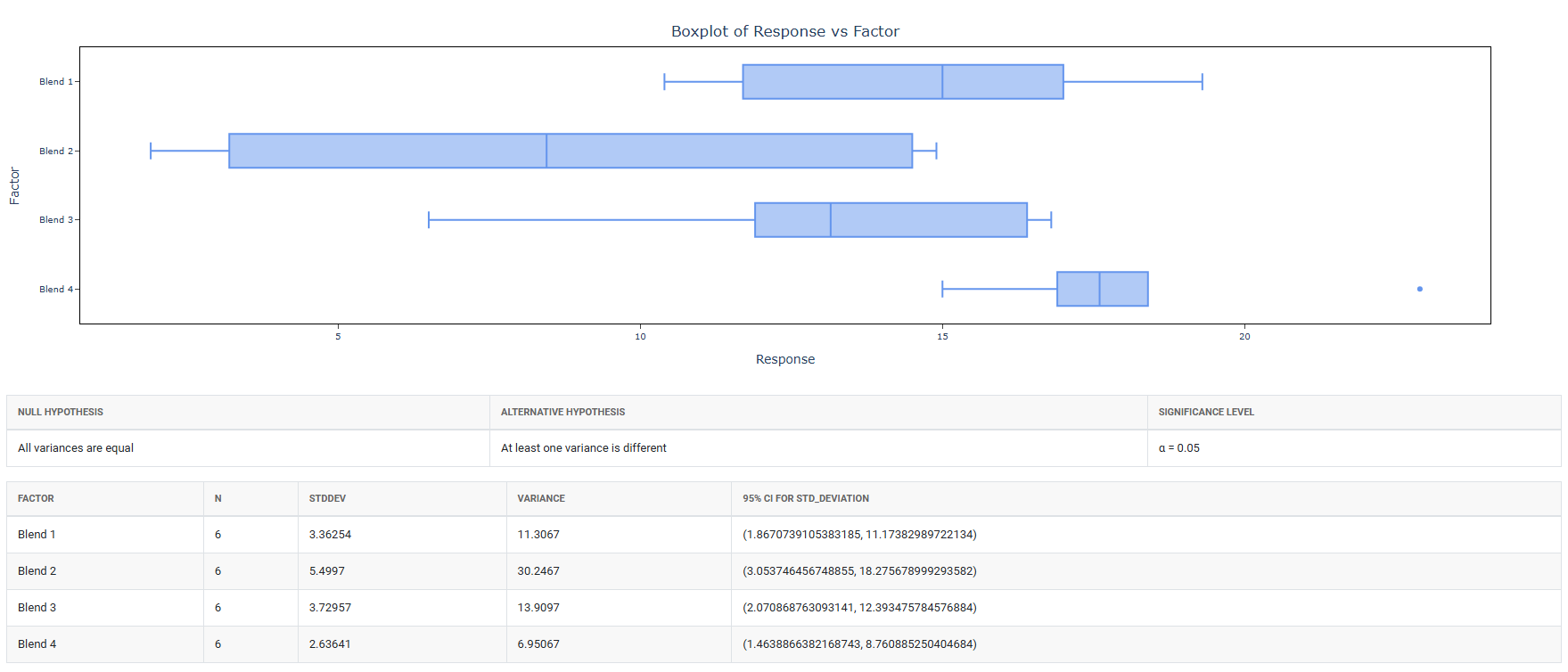
The tool checks variance homogeneity using the F-test to determine whether the two groups have statistically equal variance.

Variance Homogeneity Result	Statistical Test Applied
Variances Equal (F-test not significant)	Student’s t-test is applied. This is the standard two-sample t-test assuming equal variance across both groups.
Variances Unequal (F-test significant)	Satterthwaite’s method (Welch’s t-test) is applied. This variant does not assume equal variance and adjusts the degrees of freedom accordingly.

 

Comparing 3 or More Groups

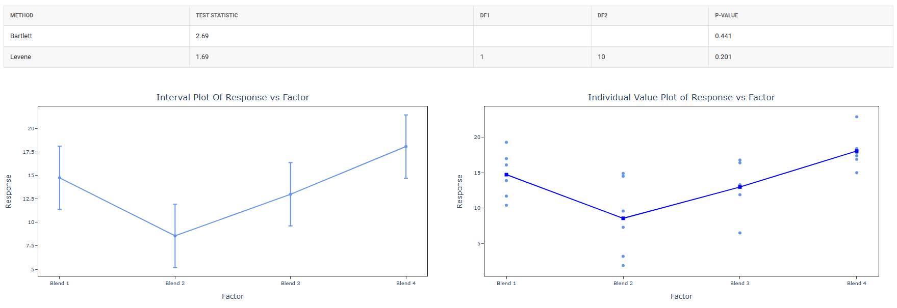
The tool checks variance homogeneity using Bartlett’s test, Levene’s test, or Brown-Forsythe test.

Variance Homogeneity Result	Statistical Test Applied
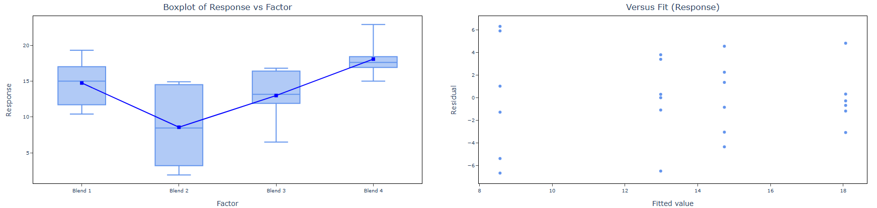
Variances Equal (not significant)	Analysis of Variance (ANOVA) is applied. → If ANOVA is significant: Dunnett’s test is performed for pairwise comparison of each treatment group against the control. → If ANOVA is not significant: No further testing is required. Stop.
Variances Unequal (significant)	The tool proceeds directly to the appropriate test that does not assume variance homogeneity.

Step 4 — Non-Parametric Pathway

When data cannot be normalised, or when data consists of counts, percentages, or ranks, the tool follows the non-parametric pathway.

Data Situation	Test Applied	Outcome / Follow-up
Count / Percentage / Rank data, ≥ 3 groups	Kruskal-Wallis test	If significant → Dunn’s test (post-hoc). If not significant → Stop.
Count / Percentage / Rank data, 2 groups	Mann-Whitney U-test	Direct comparison between two independent groups.
Categorical or indices data	Chi-Square	Test selection depends on the specific data structure and study design.

Guidelines for correct usage of OECD

• Ensure data is entered correctly and consistently data entry errors at the input stage propagate through every subsequent decision in the tree and can lead to an incorrect test being applied.
• Select response columns carefully if multiple responses are selected, each column must represent a complete, independent group dataset. If a single response is selected, ensure the factor column correctly and completely identifies every observation's group membership.
• Keep both Anderson-Darling and Shapiro-Wilk normality tests active (the default). Having two independent tests confirm the same normality conclusion strengthens the scientific defensibility of the chosen pathway.

Alternatives: When not to use OECD

• If your study does not require compliance with OECD guidelines and has no regulatory context, use the most appropriate specific statistical test directly — the OECD decision tree framework adds structured overhead that may be unnecessary for purely exploratory or academic analyses.
• If your study requires regression, correlation analysis, or dose-response modelling rather than simple group comparison, use the appropriate regression or modelling tools — the OECD tool is specifically designed for group mean comparison, not for fitting relationships between continuous variables.
• If you have paired observations  for example, before and after measurements from the same subject use paired t-test or Wilcoxon signed-rank test The OECD decision tree as implemented here assumes independent groups.
• If data is time-series or longitudinal in nature where measurements evolve over multiple sequential time points use repeated-measures ANOVA, mixed effects models, or time series analysis
• If the primary analytical goal is equivalence testing or non-inferiority assessment rather than difference detection, use dedicated equivalence testing procedures rather than the standard superiority framework of the OECD decision tree.

Example of OECD

A chemical engineer wants to compare the hardness of four blends of paint. Six samples of each paint blend were applied to a piece of metal, which was then cured. Then each sample was measured for hardness. The following steps:

1. Gathered the necessary data.

2. Now analyses the data with the help of  https://qtools.zometric.com/ or https://intelliqs.zometric.com/.

3. To find OECD choose https://intelliqs.zometric.com/> Statistical module> OECD>OECD.

4. Inside the tool, feed the data along with other inputs as follows:

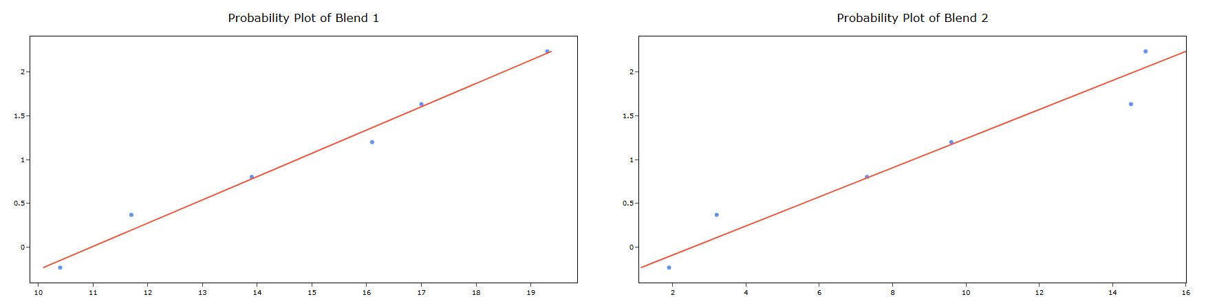
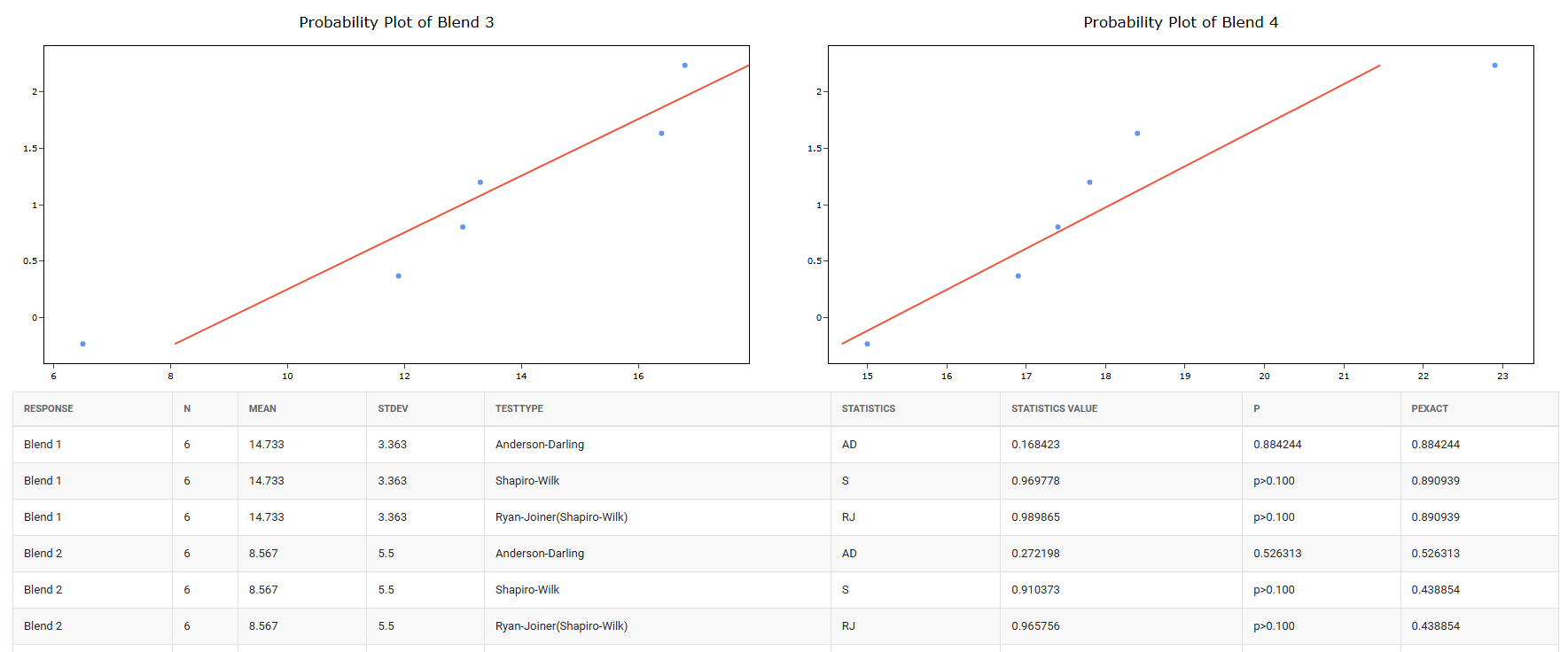
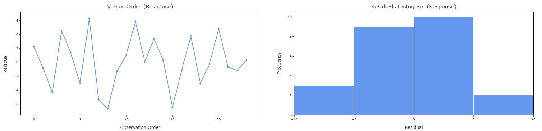
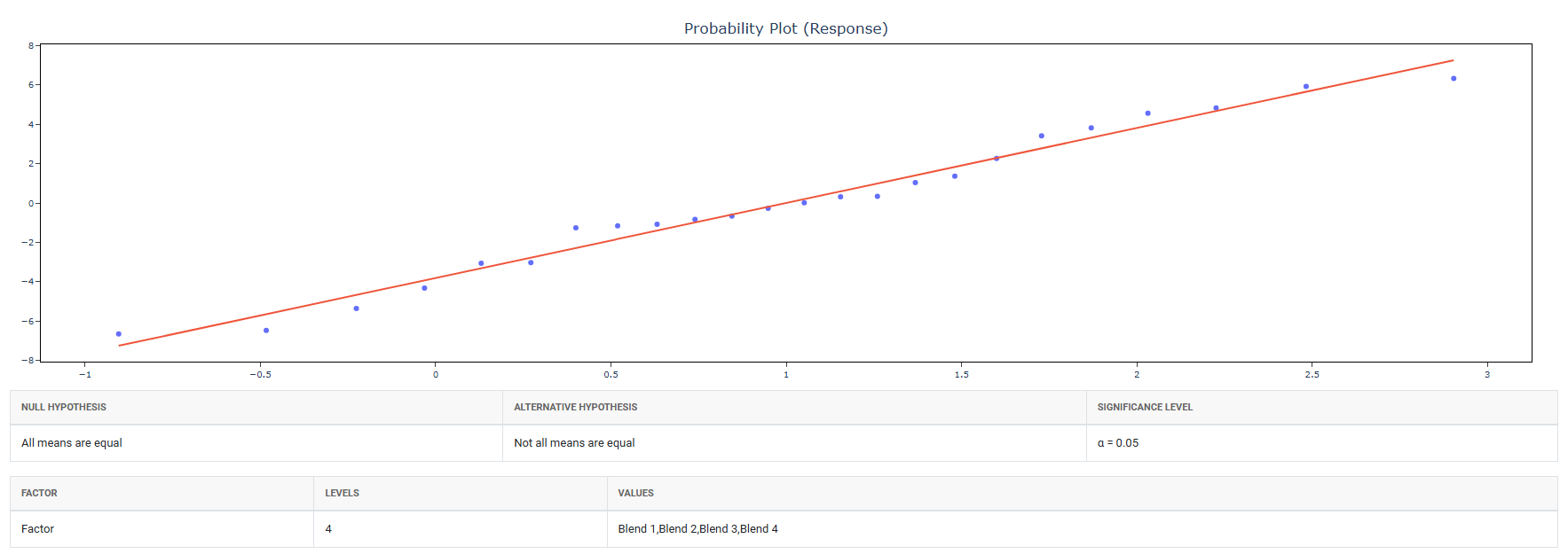
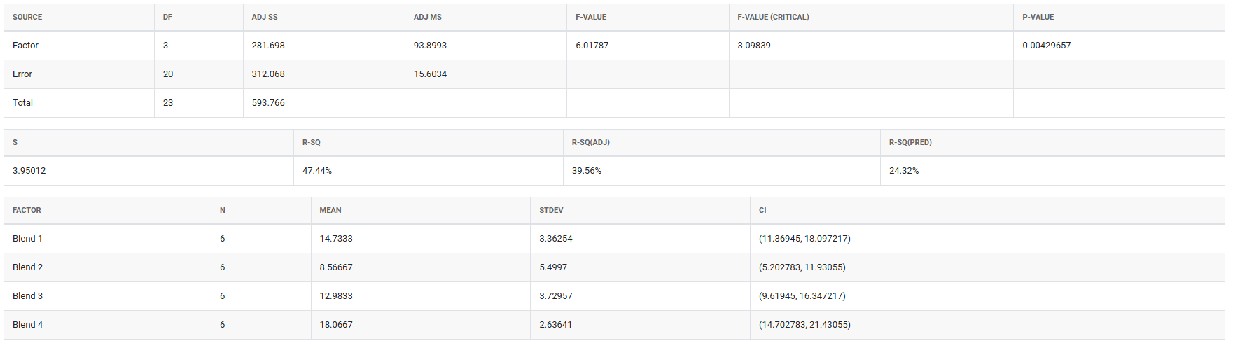
5.  After using the above mentioned tool, fetches the output as follows:

How to do OECD

The guide is as follows:

1. Login in to QTools account with the help of https://qtools.zometric.com/ or https://intelliqs.zometric.com/
2. On the home page, choose Statistical Tool> OECD>OECD.
3. Next, update the data manually or can completely copy (Ctrl+C) the data from excel sheet or paste (Ctrl+V) it or else there is say option Load Example where the example data will be loaded.
4. Next, you need to fill the required options.
5. Finally, click on calculate at the bottom of the page and you will get desired results.

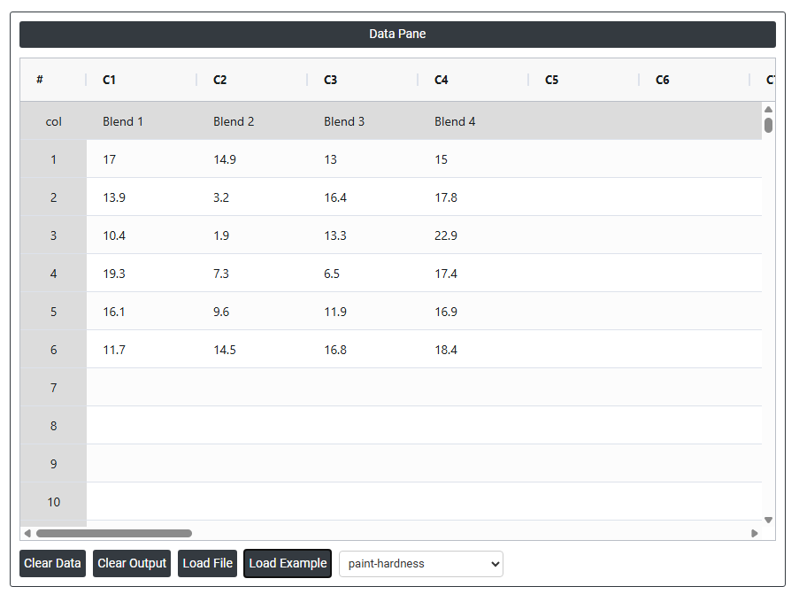
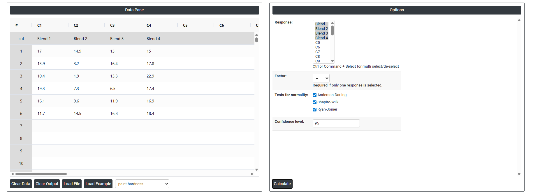
On the dashboard of OECD, the window is separated into two parts.

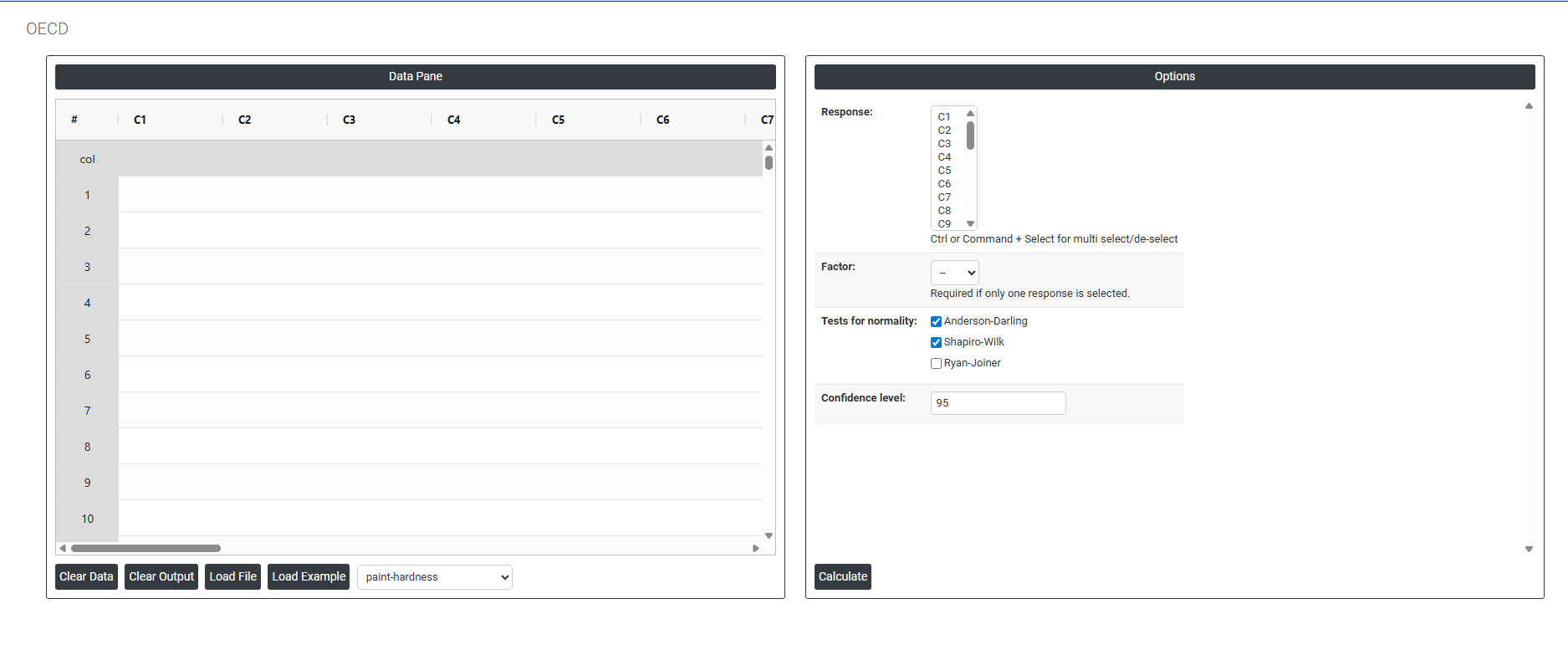
On the left part, Data Pane is present. In the Data Pane, each row makes one subgroup. Data can be fed manually or the one can completely copy (Ctrl+C) the data from excel sheet and paste (Ctrl+V) it here.

Load example: Sample data will be loaded.

Load File: It is used to directly load the excel data.

On the right part, there are many options present as follows:

• Response: Select the column or columns containing the outcome measurements you want to analyse — such as body weight, enzyme activity, tumour incidence, haematology values, or any other endpoint recorded across groups in the study. Use Ctrl or Command + Click to select multiple response columns simultaneously.

The number of response columns selected directly determines whether the Factor option is required:

Selection	How the Tool Behaves
Multiple responses selected	Each selected column represents a separate group. The tool uses the columns themselves to define the groups no additional Factor column is needed. The measurements in each column are compared against each other directly.
Single response selected	All measurements are stacked in one column and a separate Factor column must be selected to identify which group each measurement belongs to. Without the Factor column, the tool cannot determine which observations belong to which group.

⚠  Important: When a single response is selected, the Factor field becomes required. The tool will prompt you to select a Factor column before the analysis can proceed.

• Factor: Select the column that identifies the group membership of each observation. This column contains categorical labels or codes indicating which experimental group each row of data belongs to for example, Control, Low Dose, Mid Dose, High Dose, or Group 1, Group 2, Group 3. The factor column tells the tool how to split the single response column into separate groups for comparison. Without correctly specifying the factor, all measurements would be treated as belonging to the same group and no meaningful comparison could be made. This field is only required when exactly one response column is selected. When multiple response columns are selected, each column represents a group and no Factor is needed. The field will be greyed out or ignored when multiple responses are selected
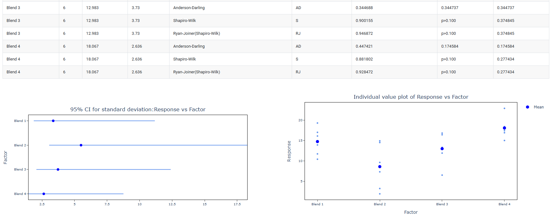
• Tests for Normality: Defines which statistical test or tests are used at Step 2 of the decision tree to assess whether the response data follows a normal distribution. The outcome of this test determines whether the parametric or non-parametric analytical pathway is followed for the entire analysis. Three tests are available:
  • Anderson-Darling : A powerful omnibus normality test that places particular emphasis on the tails of the distribution the extreme high and low values. This makes it especially sensitive to departures from normality in the tails, which are often the most practically important regions in toxicological and environmental data. The Anderson-Darling test is recommended for general-purpose use across a wide range of sample sizes and is particularly effective when tail behaviour is expected to differ from the normal distribution.
  • Shapiro-Wilk: Widely regarded as the most powerful and reliable normality test for small sample sizes — typically n < 50 — which is the most common situation in OECD guideline studies where group sizes are often 5 to 20 animals. The Shapiro-Wilk test is the primary normality test referenced in OECD statistical guidance and is the standard choice in pharmaceutical and toxicological statistics. It is strongly recommended that this test always remain active in regulatory study analyses.
  • Ryan-Joiner: A correlation-based normality test that assesses how closely the data follows the pattern expected of a normal distribution by measuring the correlation between the observed data and the theoretical normal quantiles. It is conceptually similar to the Shapiro-Wilk test but uses a different computational approach. Less commonly required in regulatory work but can be activated when a correlation-based normality assessment is specifically requested or preferred by the reviewing authority.
• When multiple normality tests are selected, the tool runs all checked tests and reports all results. The overall normality decision is based on the most conservative outcome if any selected test indicates non-normality (p < α), the data is treated as non-normal and the non-parametric pathway is followed

  Confidence Level (Default: 95): Sets the significance threshold used consistently for every hypothesis test throughout the entire decision tree including the normality test, the variance homogeneity test, and the final group comparison test. The value entered represents the percentage confidence, and the corresponding alpha (α) level used for all decisions is calculated as (100 − Confidence Level) ÷ 100.

   

  Confidence Level	Alpha Level and When to Use
  95 (default)	Alpha = 0.05. The standard confidence level for most scientific and regulatory OECD studies. There is a 5% chance of a false positive conclusion. This is the level most commonly required by OECD guidelines and regulatory authorities worldwide.
  99	Alpha = 0.01. More conservative testing requires stronger evidence before a significant result is declared. Reduces false positives but may miss smaller real effects. Use when the consequences of a false positive are particularly serious.
  90	Alpha = 0.10. More sensitive testing detects smaller differences but increases the risk of false positive conclusions. Only appropriate for exploratory or pilot studies where missing a real effect is the greater concern.