What is Principal Components?
Principal Components Analysis (PCA) is a multivariate statistical technique that reduces a large number of correlated variables into a smaller set of uncorrelated variables called principal components. Each component captures a portion of the total variation in the original dataset, with the first component explaining the most variation and each subsequent component explaining progressively less.
PCA does not discard data it mathematically transforms the original variables into a new coordinate system where each axis aligns with a direction of maximum variation. This simplifies complex, high-dimensional datasets while preserving the most meaningful patterns within them.
Simple Definitions:A technique that compresses many correlated variables into a few key components that together capture most of the variation reducing complexity while keeping the most important patterns intact.
| Term | Meaning |
| Principal Component | A new variable that is a weighted combination of original variables, capturing a specific direction of variation |
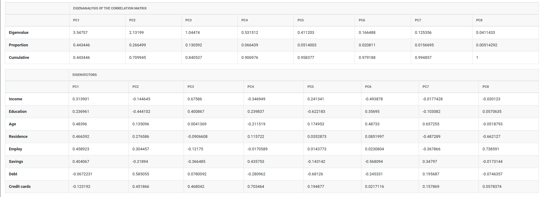
| Eigenvalue | Measures how much total variation each principal component explains |
| Scree Plot | A chart of eigenvalues in descending order, used to decide how many components to retain |
| Loadings | The contribution (weight) of each original variable to a principal component |
| Scores | The coordinates of each observation in the new principal component space |
When to use Principal Components?
- Use when you have many correlated variables and want to reduce them to a manageable number without losing key information.
- Use to identify which variables drive the most variation in a dataset.
- Use for visualizing multivariate data in two or three dimensions by plotting the first two or three components.
- Use as a preprocessing step before regression or clustering to remove multicollinearity.
- Use in quality engineering, process monitoring, and sensor data analysis where many variables are measured simultaneously.
Guidelines for correct usage of Principal Components
- All input variables should be continuous PCA is not appropriate for categorical variables.
- Standardize variables (mean = 0, SD = 1) if they are on different scales otherwise variables with larger numerical ranges will dominate the components.
- Use the scree plot and eigenvalues to decide how many components to retain a common rule is to keep components with eigenvalues greater than 1.
- Interpret components using loadings high loadings indicate which original variables are most strongly associated with each component.
- PCA identifies patterns and structure but does not explain cause and effect domain knowledge is essential to interpret component meaning.
- Aim for a sample size of at least 5 to 10 times the number of variables for stable component estimation.
Alternatives: When not to use Principal Components
- If the goal is to predict a specific response variable, use Partial Least Squares (PLS) or regression analysis instead PCA does not use a response variable.
- If variables have very low correlations with each other, PCA will not provide meaningful dimension reduction work with the original variables directly.
Example of Principal Components
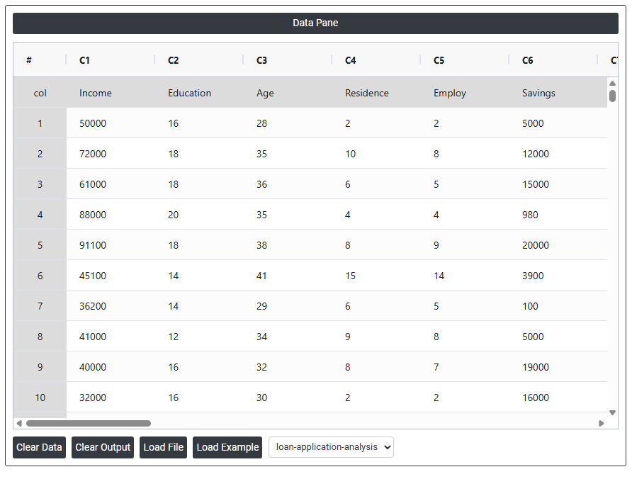
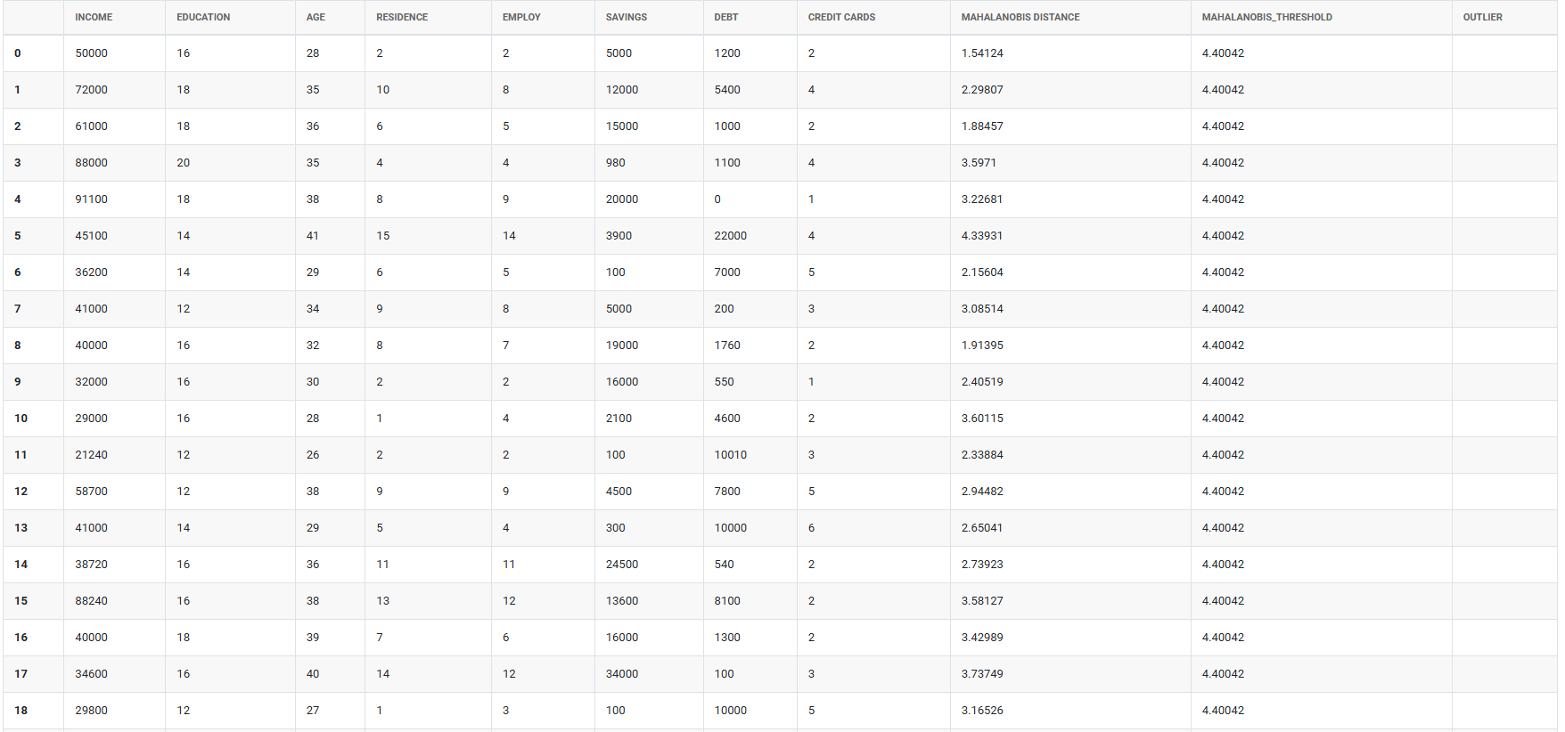
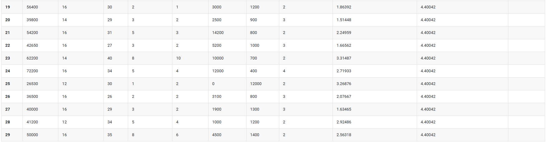
A bank requires eight pieces of information from loan applicants: income, education level, age, length of time at current residence, length of time with current employer, savings, debt, and number of credit cards. A bank administrator wants to analyze this data to determine the best way to group and report it. The administrator collects this information for 30 loan applicants. The following steps:
- Gathered the necessary data.
- Now analyses the data with the help of https://qtools.zometric.com/ or https://intelliqs.zometric.com/.
- To find Principal Components choose https://intelliqs.zometric.com/> Statistical module> Multivariate > Principal Components.
- Inside the tool, feeds the data along with other inputs as follows:
5. After using the above mentioned tool, fetches the output as follows:
How to do Principal Components
The guide is as follows:
- Login in to QTools account with the help of https://qtools.zometric.com/ or https://intelliqs.zometric.com/
- On the home page, choose Statistical Tool> Multivariate >Principal Components.
- Next, update the data manually or can completely copy (Ctrl+C) the data from excel sheet and paste (Ctrl+V) it here.
- Next, you need to fill the required options.
- Finally, click on calculate at the bottom of the page and you will get desired results.
On the dashboard of Principal Components, the window is separated into two parts.
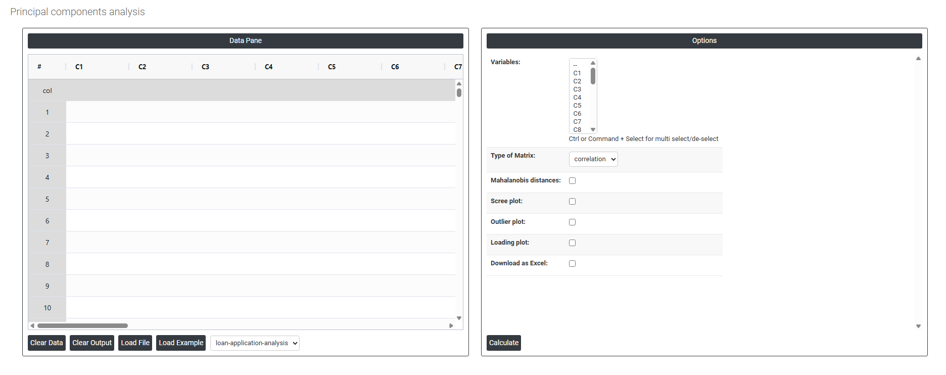
On the left part, Data Pane is present. In the Data Pane, each row makes one subgroup. Data can be fed manually or the one can completely copy (Ctrl+C) the data from excel sheet and paste (Ctrl+V) it here.
Load example: Sample data will be loaded.
Load File: It is used to directly load the excel data.
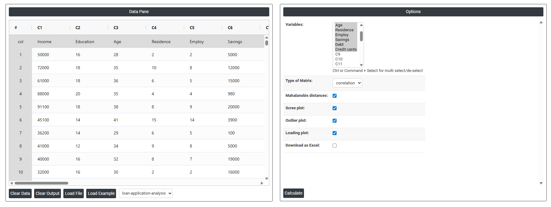
On the right part, there are many options present as follows:
- Variables: Select the columns containing the variables you want to include in the analysis. Use Ctrl or Command + Click to select multiple columns. Each selected column should be a continuous numeric variable such as income, age, debt, or savings. The more correlated these variables are with each other, the more effectively PCA will reduce them into meaningful components.
- Type of Matrix: Defines which mathematical foundation is used to calculate the principal components. Two options are typically available:
-
- Correlation Matrix — standardises all variables to the same scale (mean = 0, standard deviation = 1) before computing components. This is the recommended default when your variables are measured in different units or on very different numerical scales for example, income in thousands and age in years. Without standardisation, variables with larger ranges would dominate the components simply due to their scale, not their true importance.
- Covariance Matrix — uses the raw variances and covariances of the original variables without standardising. Only appropriate when all variables are already on the same scale and unit otherwise larger-scale variables will overwhelm the results.
- Mahalanobis Distances: When enabled, calculates the Mahalanobis distance for each observation a statistical measure of how far each data point sits from the centre of the multivariate distribution, accounting for correlations between variables. Unlike standard distance measures, Mahalanobis distance adjusts for the shape and spread of the data cloud. It is primarily used to identify multivariate outliers observations that appear unusual when all variables are considered together, even if they look normal when examined individually.
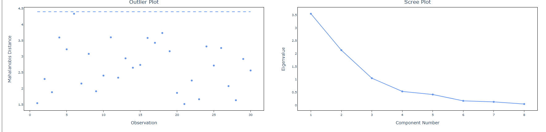
- Scree Plot: Generates a chart that plots the eigenvalue of each principal component in descending order. The scree plot is the primary tool for deciding how many components to retain. You look for the point where the line bends sharply and levels off called the elbow and retain the components above that point. A common rule is to keep components with eigenvalues greater than 1, as these explain more variance than a single original variable.
- Outlier Plot: Displays a scatter plot that helps visually identify unusual observations in the principal component space. Points that sit far from the main cluster of observations in terms of their component scores or Mahalanobis distances are flagged as potential multivariate outliers. Identifying and investigating these outliers is important before drawing conclusions from the analysis, as they can distort the components.
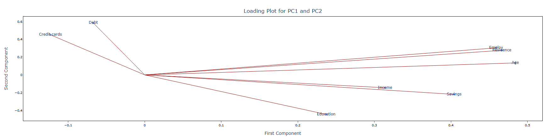
- Loading Plot: Generates a visual display of the loadings of each original variable on the principal components. Each variable is represented as a vector, and the direction and length of the vector indicate how strongly and in which direction that variable contributes to each component. Variables with long vectors pointing in the same direction are positively correlated; those pointing in opposite directions are negatively correlated. The loading plot is essential for interpreting what each principal component actually represents in terms of the original variables.
- Download as Excel: Exports the full PCA results including component scores, loadings, eigenvalues, and variance explained into an Excel file.