Two Sample t Test

What is Two Sample t Test?

When to use Two Sample t test?

• Use when you have two independent, unrelated groups and want to compare their means — for example, two machines, two suppliers, or two process settings.
• Use when the response variable is continuous — such as measurements, weights, temperatures, or dimensions.
• Use when the two groups are measured separately with no pairing or matching between individual observations.
• Use when you want to determine whether a process change, material switch, or operational difference has produced a meaningful shift in the average outcome.

Guidelines for correct usage of Two sample t test

• Each group should have data that is approximately normally distributed, or each group should contain at least 30 observations for the Central Limit Theorem to apply.
• The two groups must be independent — no observation in one group should be related to or paired with any observation in the other group.
• Check whether the two groups have equal or unequal variances before running the test — use an F test or Levene's test to assess this, as it affects which version of the t test to apply.
• Collect a sufficient sample size in each group — at least 20 to 30 observations per group is recommended for reliable results.
• Set the significance level (alpha) before collecting data — the standard default is 0.05, meaning a 5% risk of concluding a difference exists when it does not.
• Confirm that data is free from obvious outliers — extreme values can distort the mean and inflate or deflate the test result.

Alternatives: When not to use Two sample t test

• If the two groups are paired or matched (e.g. before-and-after measurements on the same subject), use Paired T Test
• If you are comparing more than two groups, use One-Way ANOVA
• If the goal is to prove that two groups are practically equivalent rather than different, use Two Sample Equivalence Test
• If data is severely non-normal and sample sizes are small, use Mann-Whitney Test (a non-parametric alternative) instead.
• If you only have summarised data (mean, SD, n) rather than raw observations, use Two Sample T Test (Summarized)

Example of Two sample t test?

An economist collects data on the monthly energy cost for 25 families in the current year to determine if there has been a change from the previous year when the mean cost was $200. They perform a One sample t test to test if the current year's energy cost is significantly different from $200. The test in following steps:

1. Gathered the necessary data.

2.  Now analyses the data with the help of  https://qtools.zometric.com/ or https://intelliqs.zometric.com/.
3.  To find One sample t-test choose https://intelliqs.zometric.com/> Statistical module> Hypothesis Test> Two sample t-test.
4.  Inside the tool, feeds the data along with other inputs as follows:

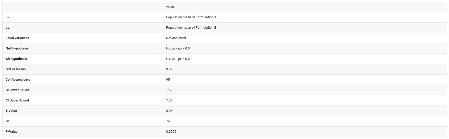
5. After using the above mentioned tool, fetches the output as follows:

How to do Two sample t test

The guide is as follows:

1. Login in to QTools account with the help of https://qtools.zometric.com/ or https://intelliqs.zometric.com/
2. On the home page, choose Statistical Tool> Hypothesis Test >Two sample t test .
3. Next, update the data manually or can completely copy (Ctrl+C) the data from excel sheet and paste (Ctrl+V) it here.
4. Next, you need to put the values of confidence level and hypothesized mean.
5. Finally, click on calculate at the bottom of the page and you will get desired results.

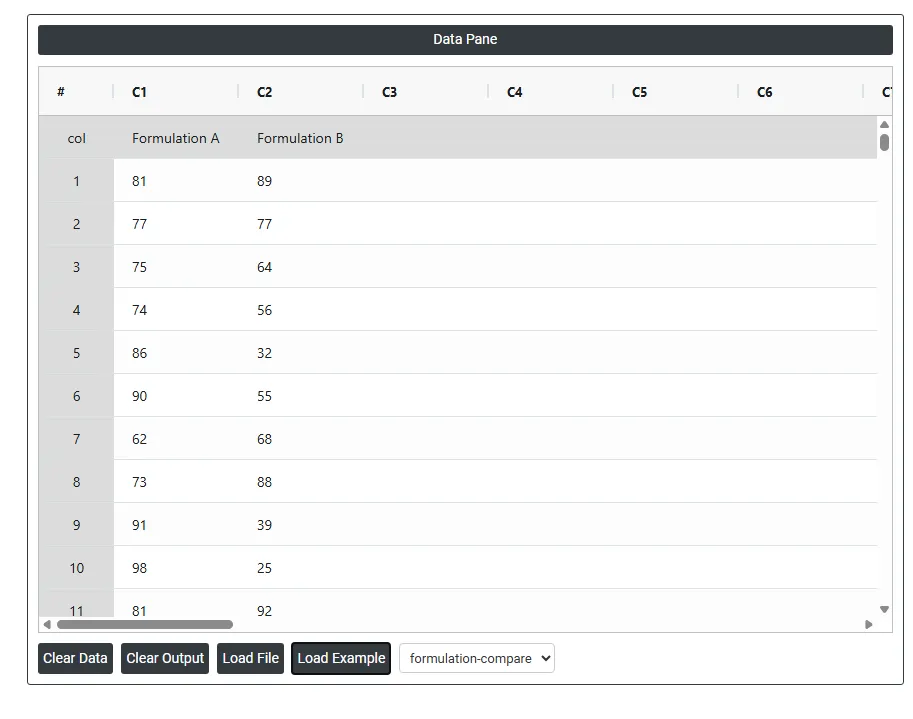
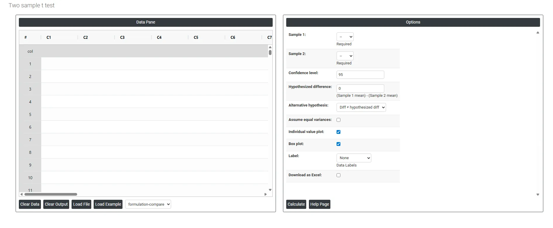
On the dashboard of Two sample t test, the window is separated into two parts.

On the left part, Data Pane is present. In the Data Pane, each row makes one subgroup. Data can be fed manually or the one can completely copy (Ctrl+C) the data from excel sheet and paste (Ctrl+V) it here.

Load example: Sample data will be loaded.

Load File: It is used to directly load the excel data.

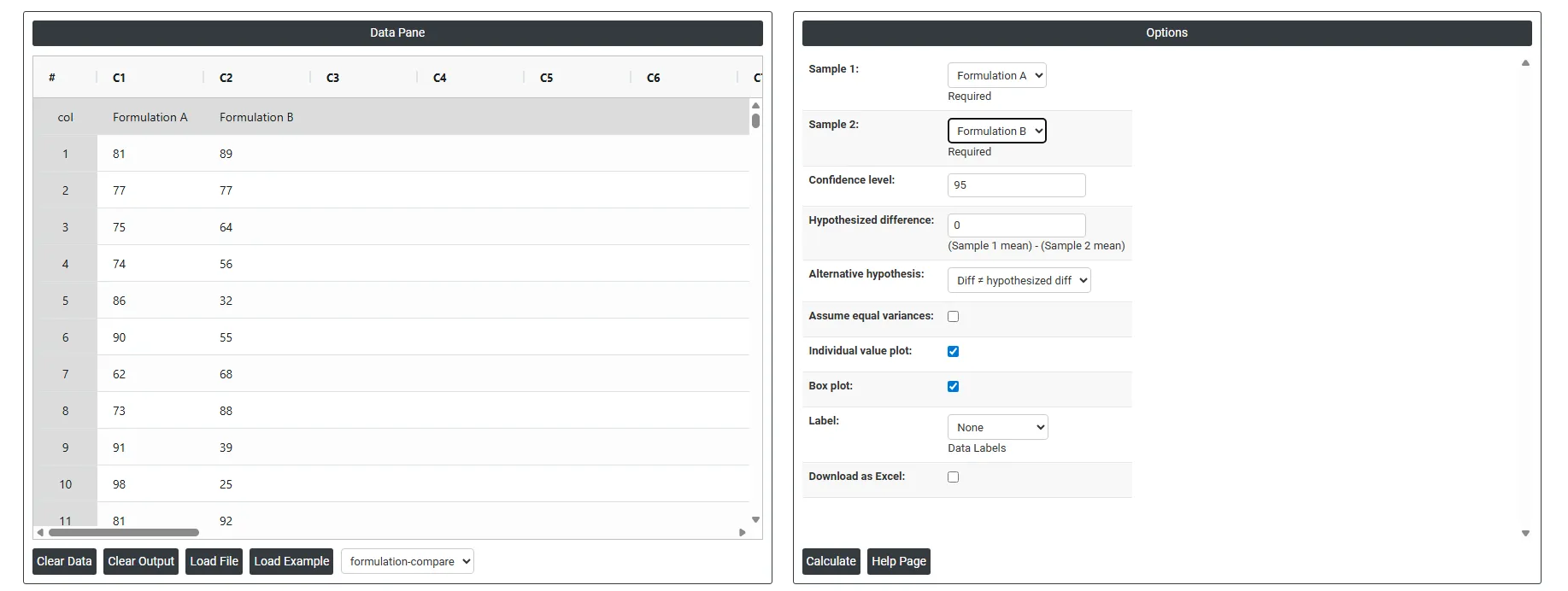
On the right part, there are many options present as follows:

• Sample 1: Select the column containing the data for the first group you want to compare — for example, measurements from Machine A, Supplier 1, or Formulation A. This is a required field and must contain continuous numerical values.
• Sample 2: Select the column containing the data for the second group — for example, measurements from Machine B, Supplier 2, or Formulation B. This is also required and must be independent of Sample 1, meaning the two datasets have no pairing or matching between individual observations.
• Confidence Level: Sets the certainty level for the confidence interval calculated around the difference between the two means. The standard default is 95%, meaning you are 95% confident the true difference between the two group means falls within the displayed interval. A higher confidence level (e.g. 99%) produces a wider interval; a lower level (e.g. 90%) produces a narrower one.
• Hypothesized Difference: The value you are testing against — representing the expected or assumed difference between the two group means (Sample 1 mean minus Sample 2 mean). Setting this to 0 tests whether the two means are equal. Setting it to any other value tests whether the difference equals that specific amount — for example, entering 5 tests whether Group 1 averages exactly 5 units more than Group 2.
• Alternative Hypothesis; Defines the direction of the test — what you are trying to prove about the difference between the two means. Three options are available:

• Diff ≠ Hypothesized Diff — a two-tailed test that checks whether the difference is simply not equal to the hypothesized value, in either direction. Use when you have no prior expectation about which group will be larger.
• Diff < Hypothesized Diff — a one-tailed test that checks whether the actual difference is smaller than the hypothesized value. Use when you specifically expect Sample 1 to be lower than Sample 2.
• Diff > Hypothesized Diff — a one-tailed test that checks whether the actual difference is larger than the hypothesized value. Use when you specifically expect Sample 1 to be higher than Sample 2.

• Assume Equal Variances: When checked, the test assumes both groups have the same underlying population variance and uses a pooled standard deviation to calculate the test statistic — producing a slightly more powerful test when the assumption holds. When unchecked, the test uses separate variance estimates for each group (Welch's t test), which is more reliable when the two groups have noticeably different spreads. If you are unsure, leave this unchecked as it is the safer and more conservative approach.
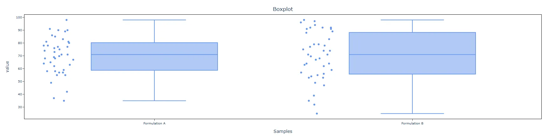
• Individual Value Plot: When enabled, displays a plot showing every individual data point for both groups side by side. This gives a clear view of the full data distribution, spread, and any unusual values — making it easier to visually assess whether the two groups differ and whether any outliers are present.
• Box Plot: When enabled, displays a box-and-whisker plot for each group, summarising the median, interquartile range, and overall spread. Box plots are useful for comparing the centre and variability of the two groups at a glance and for spotting skewness or outliers that may affect the test results.
• Label: Controls what additional information is displayed on the Individual Value Plot or Box Plot. Options include:

• None — no extra labels on the plot
• Outliers — highlights only statistically extreme data points
• Individual Data — labels each plotted data point
• All Quartiles — displays Q1, median, and Q3 values
• Means — marks the mean of each group on the plot
• Data Labels — displays the actual values for plotted points

• Download as Excel: Exports the test results, summary statistics, confidence intervals, and p-value into an Excel file. This is useful for including the results in reports, sharing with colleagues, or keeping a formal record of the analysis.