
Paired t test
The paired t-test, also known as the dependent sample t-test, is used to evaluate whether there is a significant difference between the means of two related groups. This test is applied when each subject or unit is measured twice, under different conditions or at different times, creating pairs of observations.
Last reviewed
Key takeaway
The paired t-test, also known as the dependent sample t-test, is used to evaluate whether there is a significant difference between the means of two related groups.
On this page
What is Paired t test?
The paired t-test, also known as the dependent sample t-test, is used to evaluate whether there is a significant difference between the means of two related groups. This test is applied when each subject or unit is measured twice, under different conditions or at different times, creating pairs of observations. The paired t-test assesses whether the mean difference between these paired observations is significantly different from zero. The null hypothesis assumes that the mean difference is zero, while the alternative hypothesis posits that the mean difference is not zero.
The paired t-test is particularly useful for before-and-after studies or any situation where two measurements are taken from the same subjects, allowing researchers to determine if observed changes are statistically significant.
When to use Paired t test?
A paired t test is used when the two samples being compared are related or paired, such as in a before-and-after study, where the same individuals are measured twice, or in a matched-pairs study, where individuals are matched on important characteristics and then assigned to different treatments.
- Normal Distribution: The differences between paired observations should be approximately normally distributed.
- Random Sampling: The pairs should be randomly selected.
- Independence: Each pair should be independent of other pairs, and the differences within pairs should be independent of each other.
Here are some specific situations where a paired t-test might be appropriate:
- Before-and-after studies: When you want to test if an intervention or treatment has had a significant effect on an individual or group, a paired t-test can be used to compare the mean scores of the same group before and after the intervention.
- Matched-pairs studies: In studies where individuals are paired based on similar characteristics, such as age, sex, or health status, and then assigned to different treatments, a paired t-test can be used to compare the means of the two groups.
- Repeated-measures studies: When a study involves measuring the same variable multiple times on the same individual or group, a paired t-test can be used to compare the means of the measurements at different time points.
Guidelines for correct usage of Paired t test
- Continuous data can take on an infinite number of values between any two points.
- Sample sizes should be greater than 20.
If sample size is greater than 20 and the distribution is unimodal and continuous, the test remains valid even with mild skewness.
For sample sizes less than 20, graph the data to check for skewness and unusual observations. Exercise caution if the data is severely skewed or contains many outliers. - Ensure you have paired (dependent) observations, such as repeated measurements on the same item under different conditions.
- For independent observations between two samples, use the 2-Sample t-test instead.
- Collect data randomly to make generalizations about the population.
- Determine an appropriate sample size that provides enough precision and protection against errors.
Alternatives: When not to use Paired t test
- In case you have two sets of independent observations, it is recommended to use the 2-Sample t-test instead.
Example of Paired t test?
Example 1
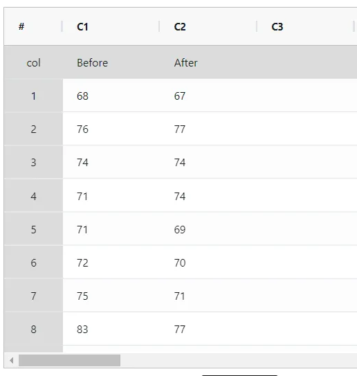
A physiologist wants to determine whether a particular running program has an effect on resting heart rate. The heart rates of 20 randomly selected people were measured. After one year on the running program, the heart rates of the same individuals were measured again. This resulted in a pair of observations (before and after) for each person. A paired t-test was then carried out to assess whether there is a statistically significant difference in heart rates before and after the running program. The test was performed following these steps:
- Gathered the necessary data.
- Now analyses the data with the help of https://qtools.zometric.com/ or https://intelliqs.zometric.com/.
- To find Paired t-test choose https://intelliqs.zometric.com/> Statistical module> Graphical analysis> Paired t-test.
- Inside the tool, feeds the data along with other inputs as follows:
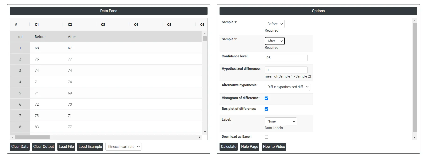
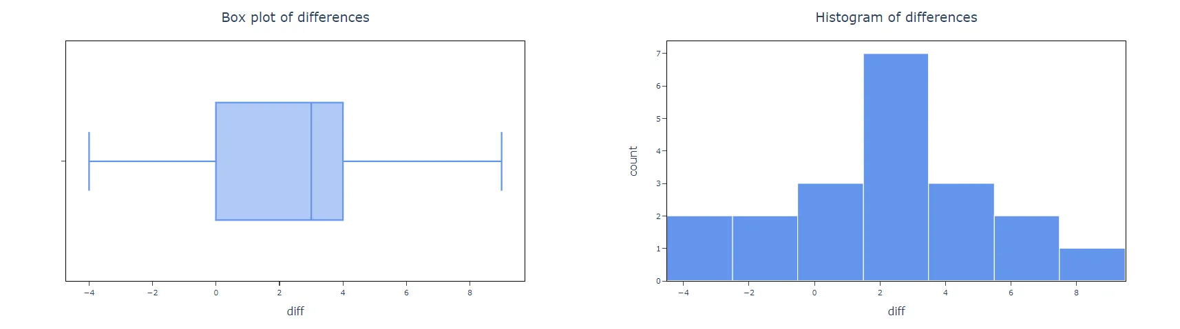
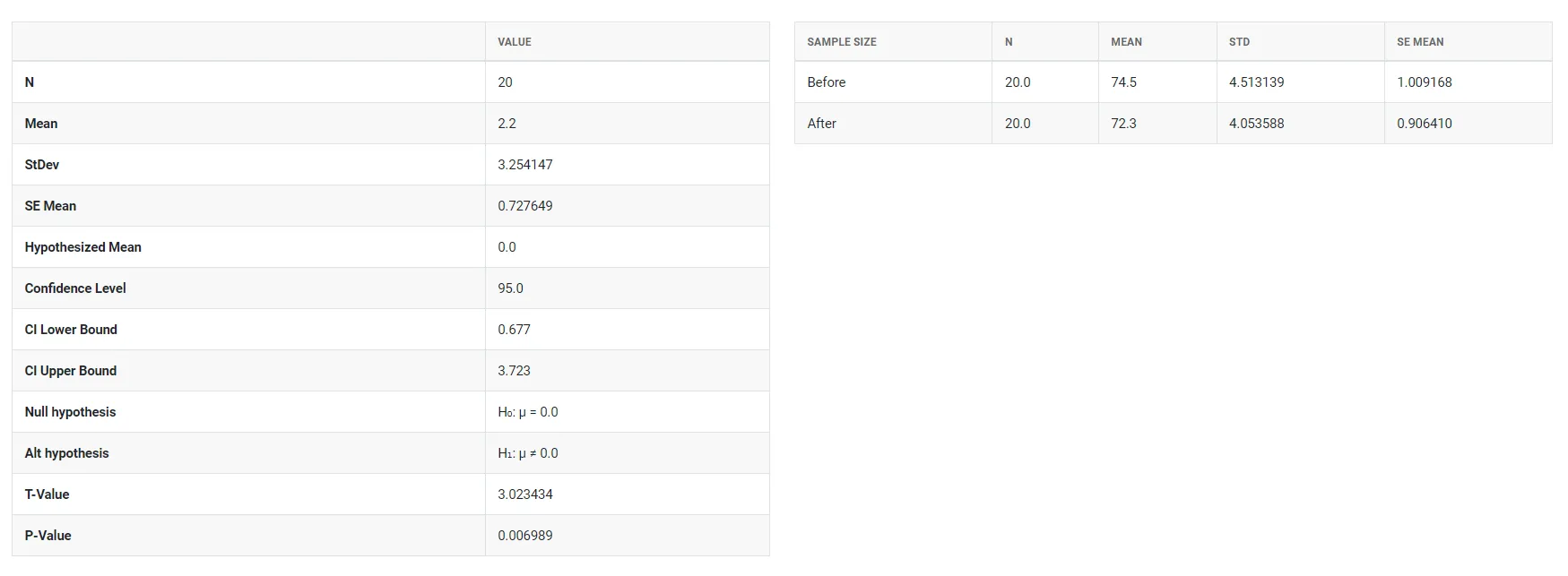
5. After using the above mentioned tool, fetches the output as follows:
How to do Paired t test
The guide is as follows:
- Login in to QTools account with the help of https://qtools.zometric.com/or https://intelliqs.zometric.com/
- On the home page, choose Statistical Tool> Graphical analysis > Paired t test
- Click on Paired t test and reach the dashboard.
- Next, update the data manually or can completely copy (Ctrl+C) the data from excel sheet and paste (Ctrl+V) it here.
- Next, you need to put the values of confidence level, and hypothesized difference.
- Finally, click on calculate at the bottom of the page and you will get desired results.
On the dashboard of Paired t test, the window is separated into two parts.
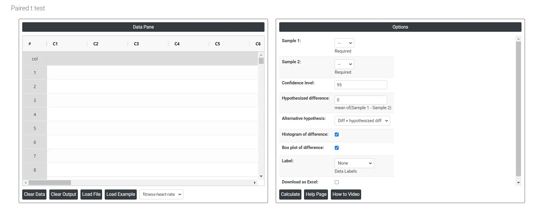
On the left part, Data Pane is present. In the Data Pane, each row makes one subgroup. Data can be fed manually or the one can completely copy (Ctrl+C) the data from excel sheet and paste (Ctrl+V) it here.
Load example: Sample data will be loaded.
Load File: It is used to directly load the excel data.
On the right part, there are many options present as follows:
- Confidence level:In hypothesis testing, the confidence level represents the degree of certainty or level of confidence that we have in our statistical analysis. It is a probability value that indicates the likelihood that the true population parameter falls within the specified range of values.Typically, the confidence level is expressed as a percentage and is denoted by (1 - α), where α is the level of significance or the probability of rejecting a true null hypothesis. For example, if we have a confidence level of 95%, then we are saying that we are 95% confident that the true population parameter lies within our interval estimate, and there is a 5% chance of making a type I error (rejecting a true null hypothesis).In practical terms, a higher confidence level means that we are more confident in our statistical analysis and results. However, increasing the confidence level also increases the width of the confidence interval, making it more difficult to detect small effects. Therefore, the choice of the confidence level depends on the context of the study and the goals of the researcher.
- Hypothesized difference: The hypothesized difference refers to the difference in the population parameters between the null hypothesis and the alternative hypothesis. For example, if we want to test whether the mean score on a test is significantly different between two groups (e.g., males and females), the hypothesized difference would be the difference between the mean score of males and the mean score of females.
- Alternative hypothesis: In hypothesis testing, the alternative hypothesis (also called the research hypothesis) is a statement that represents a different conclusion than the null hypothesis. The null hypothesis typically represents the status quo or the assumption that there is no significant difference or relationship between two or more groups or variables. The alternative hypothesis is the statement that is being tested, and it proposes that there is a significant difference or relationship between the groups or variables being studied.
- Histogram of difference:The histogram of differences is a graphical representation of the distribution of differences between two sets of data. In the context of hypothesis testing, it can be used to visually assess the difference between the means of two groups.The process typically involves collecting data from two groups, calculating the mean and variance for each group, and then calculating the difference between the means. This difference is often referred to as the "effect size".
- Individual value plot of difference:An individual value plot of difference is a graphical representation of the differences between two groups in a hypothesis test. In a hypothesis test, researchers want to determine if there is a statistically significant difference between two groups, such as a treatment group and a control group.An individual value plot can be used to display the differences between the two groups on a single plot. The plot typically shows the individual data points for each group, as well as the mean and standard deviation for each group.
- Box Plot of difference: In the context of hypothesis testing, a box plot of difference can be used to display the distribution of the differences between two groups being compared. For example, if we are comparing the mean values of two groups, we can calculate the difference between the means and then create a box plot of the differences.
- Histogram of difference: Check in will provide you histogram chart or else not.
- Label: This will do the data labels, which contains three options:
- Outlier: Data values that are far away from other data values, can strongly affect your results.
- All quartiles: Quartiles are values that divide a sample of data into four equal parts. Quickly evaluate a data set's spread and central tendency.
- Mean: The mean in a box plot to provide additional information about the data's central tendency.
- Individual Data: An individual data point is a single observation or value in a dataset.
- Download as Excel: This will display the result in an Excel format, which can be easily edited and reloaded for calculations using the load file option.