Advanced Stability Study (ICH Compliant)

What is Advanced Stability Study?

The Advanced Stability Study is Zometric's ICH Q1E-compliant tool for estimating the shelf life of a pharmaceutical or other regulated product. Like the basic Stability Study tool, it fits a regression model of a measurable response (potency, concentration, pH, moisture, etc.) against time, and finds the point at which the response is predicted to cross a specification limit. The Advanced version extends this with the full set of ICH Q1E capabilities needed for a regulatory submission: batch poolability testing (fixed or random batch effects), an optional non-batch factor (e.g. strength or container/closure system) with its own poolability test, bracketing and matrixing design handling, an ICH Q1E Appendix A extrapolation assessment based on storage condition and significant-change history, Box-Cox response transformation, temperature projection using Arrhenius or Q10 kinetics (so a shelf life estimated at one storage condition can be projected to another temperature), and an overage calculator that computes how much excess active ingredient to add at manufacture so the product still meets its lower specification at the end of the target shelf life.

In short: use the plain Stability Study tool for a quick shelf-life estimate from time/response/batch data; use the Advanced Stability Study tool when the study needs to satisfy ICH Q1E documentation requirements, involves multiple temperatures, or requires an overage recommendation.

When to use Advanced Stability Study?

Data Requirements

• The dataset must include a time variable as the primary predictor — this is what drives the analysis (e.g. 0, 3, 6, 9, 12, 18, 24 months).
• An optional batch factor can be included to account for differences across production batches; it can be treated as a Fixed factor, a Random factor, or omitted entirely ("No batch factor").
• An optional non-batch factor (Factor2) can be included for ICH Q1E multi-factor studies — for example, strength, container/closure type, or orientation — and is tested for poolability separately from batch, at a fixed α = 0.05.
• An optional Temperature column can be included when the study covers more than one storage temperature. When supplied, the tool derives the activation energy (Ea) directly from the data using an Arrhenius fit, instead of requiring you to type in a literature value.
• The response variable must be continuous — for example, potency, concentration, pH, or weight.

Data Collection Guidelines

• Ensure the data accurately represents the batches/population of interest — incomplete or biased data leads to unreliable shelf life estimates.
• Collect sufficient data points across multiple time intervals (ICH Q1E typically expects a minimum cadence — e.g. 0, 3, 6, 9, 12, 18, 24, 36 months) to provide the precision needed for accurate predictions and for the ANCOVA/pooling tests to have adequate power.
• If a bracketing or matrixing design was used, record which levels/combinations were actually tested — the tool has dedicated options to document this and to apply the correct ICH Q1E Appendix C caveats to the reported shelf life.
• If multiple storage temperatures were tested for a kinetics/Arrhenius projection, record the exact temperature (°C) alongside each observation in the Temperature column.
• Measure all variables as accurately and precisely as possible — measurement errors directly affect the quality of the model and of any temperature projection.
• Record data in the order it is collected to preserve the time-based structure of the analysis.

Model Fit

• The model must provide a good fit to the data — a poorly fitting model will produce misleading shelf life estimates and unreliable Arrhenius/Q10 projections.
• After fitting, review the ANOVA/Model Selection table (which terms were retained by the batch-pooling and factor2-pooling tests), the residual plots, the diagnostic statistics for unusual observations, and the Model Summary (S, R-sq, R-sq(adj), R-sq(pred)) to confirm the model represents the data well.
• If a Kinetics/Transform Mismatch warning appears, reconsider the combination of Box-Cox transform and Degradation Kinetics model before trusting the projected shelf lives at other temperatures.

Guidelines for correct usage of Advanced Stability Study

• Use a continuous response variable such as potency, concentration, or moisture content; categorical responses are not suitable for this analysis.
• Always include a time variable as the predictor — the entire analysis is built around tracking change over time.
• Include a batch factor when multiple production batches are being studied, and decide whether to treat it as Fixed (specific batches of interest) or Random (batches representative of a larger population) based on the study objective.
• Leave Alpha for Pooling Batches at its ICH Q1E default of 0.25 unless you have a specific reason to change it — this deliberately liberal threshold makes it harder to justify pooling batches together, which keeps the shelf life estimate conservative.
• Use the Non-batch factor (Factor2) field only for a genuine ICH Q1E multi-factor study (e.g. strength or container type) — it is tested for poolability at the conventional α = 0.05, not the batch-pooling α.
• Only fill in the Temperature column if the study genuinely spans multiple storage temperatures; doing so automatically switches the Kinetics model to Arrhenius and derives Ea from your data rather than from a manually entered value.
• Make sure the Degradation Kinetics selection matches the Box-Cox transform: zero-order kinetics assumes no transform, while first-order kinetics assumes a natural-log transform (λ = 0). A mismatch triggers a Kinetics / Transform Mismatch warning and can make Arrhenius/Q10 projections unreliable.
• Only enable Overage for a degrading product (a negative slope) with a Lower Spec entered — the tool will refuse to calculate overage otherwise, since overage only makes sense when potency/response is expected to fall over time.
• If the study used a bracketing or matrixing design, check the corresponding option and describe it — the report will then include the correct ICH Q1E Appendix C disclaimers about extending the shelf life to untested levels or combinations.
• Record the Storage condition and any Significant change observations at the accelerated and intermediate conditions — these drive the ICH Q1E Appendix A extrapolation assessment that caps how far the calculated shelf life may be extrapolated beyond the longest available time point.
• Gather enough data points across sufficient time intervals to support statistically reliable estimates and reduce prediction uncertainty.
• Measure all variables with maximum precision — even small measurement errors can shift the estimated shelf life significantly.
• Record observations in the order they are collected to maintain the integrity of the time-series structure.
• After fitting the model, always validate it using the residual plots, the Model Summary, and the ICH Q1E extrapolation assessment before drawing conclusions or reporting a shelf life.
• A poor model fit, an unresolved kinetics/transform mismatch, or an extrapolation-cap warning are all signals to reconsider the model, check for outliers, or re-examine the data before proceeding.

Alternatives: When not to use Advanced Stability Study

• If the study does not need ICH Q1E documentation (no bracketing/matrixing, no temperature projection, no overage) and you just need a quick shelf-life number, use the simpler Stability Study tool instead — it exposes the same core regression/pooling engine with a shorter, easier options list.
• If there is no time variable in the data, use Fit Regression Model instead to analyze the relationship between other continuous predictors and the response.
• If the goal is to predict a response from multiple non-time predictors, use Fit Regression Model for multi-variable analysis.
• If the response variable has two categories such as pass or fail, use Fit Binary Logistic Model instead.
• If the response variable contains three or more ordered categories such as low, medium, or high, use Ordinal Logistic Regression instead.
• If the response variable contains three or more unordered categories such as scratch, dent, or tear, use Nominal Logistic Regression instead.

Example of Advanced Stability Study?

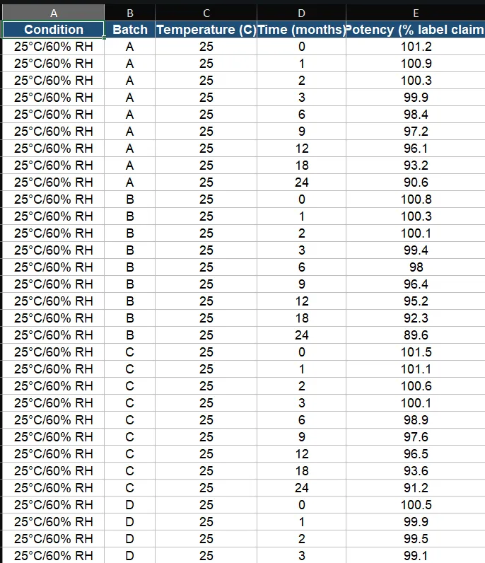
A pharmaceutical company's quality engineer wants to establish the shelf life of a new tablet formulation, and additionally wants to know how that shelf life would change if the product were stored at a warmer temperature. The drug's potency declines gradually over time. Five pilot batches are available, tested at nine time points at the intended long-term storage condition (25°C/60%RH), and a subset of the same batches was additionally tested at an accelerated condition (40°C) to support an Arrhenius projection. Each batch is treated as a Fixed factor, since all batches are systematically sampled. The lower specification is entered as 90 (i.e. the product must retain at least 90% of label claim). Overage is also enabled so the engineer can see how much extra drug substance should be added at manufacture to guarantee 90% potency through the proposed 24-month shelf life. The following steps were used:

1.      Gathered the necessary time, batch, response (potency), and temperature data.

2.      Analyzed the data using https://statsai.zometric.com/ .

3.      To find Advanced Stability Study, chose https://statsai.zometric.com/ > Statistical module > Regression > Advanced Stability Study.

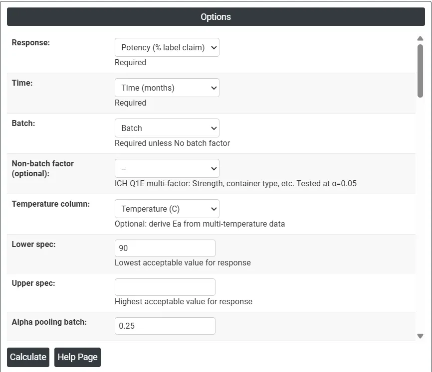
4.      Inside the tool, fed the data along with the other inputs — Response = Potency, Time = Time, Batch = Batch, Temperature = Temperature, Lower Spec = 90, Batch is = Fixed factor, Kinetics model = Arrhenius, Reference temperature = 25, Target temperatures = 5, 25, 30, 40, Overage = checked, Label Claim = 100, Target Shelf Life = 24 — as follows:

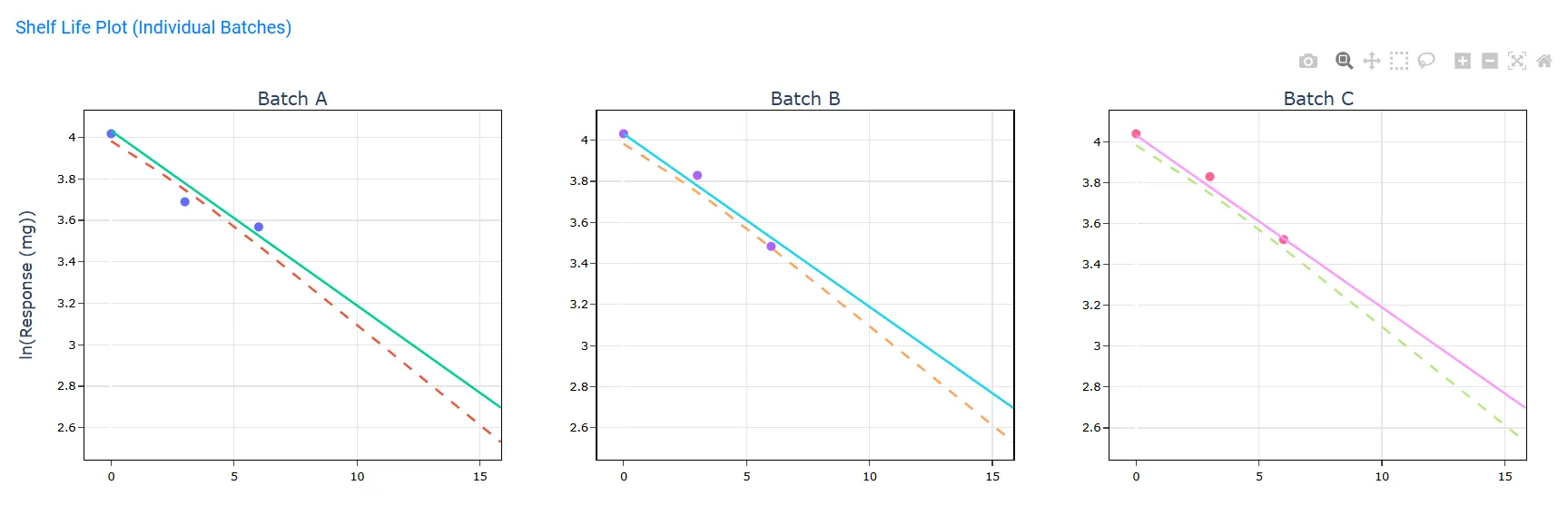
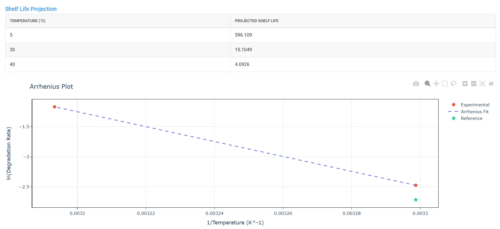
5.      After using the tool, the following output was produced — the shelf-life estimate, the ANOVA/pooling decision, the shelf-life plot, the Arrhenius projection to other temperatures, and the overage recommendation:

How to do Advanced Stability Study

The guide is as follows:

6.      Login to Stats AI account with the help of https://statsai.zometric.com/

7.      On the home page, choose Statistical Tool > Regression > Advanced Stability Study.

8.      Next, update the data manually or completely copy (Ctrl+C) the data from an excel sheet and paste (Ctrl+V) it, or use the Load Example option where the example data will be loaded, or use Load File to directly load an excel/csv file.

9.      Next, fill in the required options — described field by field below.

10.   Finally, click Calculate at the bottom of the page and you will get the desired results.

On the dashboard of Advanced Stability Study, the window is separated into two parts.

Data Pane (left part)

On the left part, the Data Pane is present. Data can be fed manually, or you can completely copy (Ctrl+C) the data from an excel sheet and paste (Ctrl+V) it here. As soon as data is present, the Response, Time, Temperature, Batch, and Non-batch factor dropdowns on the right automatically filter themselves down to only the columns that actually contain data, labelled using whatever header text you typed in the first row of that column.

• Load Example: Loads a sample drug shelf-life dataset so you can see the tool working end to end before using your own data.
• Load File: Lets you directly upload an Excel or CSV file instead of pasting data into the grid.
• Clear Data / Clear Output: Clear Data empties the Data Pane; Clear Output clears the results panel below, without touching the entered data or options.

Options (right part)

On the right part, there are many options present, grouped below by purpose.

Core variables

• Response: The measurement you are tracking over time, such as potency, pH, or moisture content. This is the variable being tested to see whether the product remains within acceptable limits throughout its shelf life.
• Time: The time points at which each measurement was recorded (e.g. 0, 3, 6, 12 months). The tool uses this variable to model how the response changes over the storage period.
• Batch: The specific production batch each sample belongs to. Including batch lets the tool detect whether different batches degrade at different rates, which directly affects the shelf life estimate. Required unless "Batch is" is set to "No batch factor".
• Non-batch factor (optional): An ICH Q1E multi-factor column such as Strength or Container type. It is tested for poolability independently of Batch, at a fixed significance level of α = 0.05, and its poolability verdict (poolable / common slope / not poolable) is reported separately.
• Temperature column: Optional. When your study covers more than one storage temperature, assign that column here to let the tool derive the Arrhenius activation energy directly from your data. Selecting a Temperature column automatically switches the Kinetics model to Arrhenius and disables the manual Activation Energy / Q10 entry fields, since those values are now computed for you.

Specification limits and batch pooling

• Lower Spec: The minimum acceptable value for the response. If the product's measurement falls below this limit, it is considered out of specification and no longer safe or effective for use.
• Upper Spec: The maximum acceptable value for the response. If the measurement exceeds this limit, the product is again considered out of specification. Depending on the product, you may use one or both spec limits — at least one of Lower Spec / Upper Spec must be entered.
• Alpha for Pooling Batches: Controls whether batches are analyzed separately or combined (pooled) into one model. A higher alpha value (default 0.25) makes it harder to pool batches, which gives a more conservative and reliable shelf life estimate. The default of 0.25 is intentionally higher than the typical 0.05 used in hypothesis testing — in stability studies it is safer to keep batches separate unless there is strong evidence they behave the same way. The same tests decide, in order: whether the degradation rate (slope) differs across batches, and if not, whether only the starting point (intercept) differs — the least complex model that still fits is the one reported.
• Use One Spec Limit to Calculate Shelf Life: Some products degrade in only one direction — for example, potency only decreases over time. In such cases only one spec limit (lower or upper) is actually relevant to the shelf life calculation. Enabling this option tells the tool to spend its full confidence budget on that single boundary rather than splitting it between both limits, giving a more accurate estimate. The tool automatically determines whether the lower or the upper limit is the relevant one from the direction of the fitted trend.

Batch treatment

• Batch is: Defines how the batch variable is treated statistically. "No batch factor" ignores batch and fits a single pooled regression line. "Fixed factor" means the results apply only to the specific batches tested — the shelf life is estimated from those exact batches (and is reported as the minimum across batches). "Random factor" treats the tested batches as a sample from a larger population of future batches and fits a mixed-effects model instead, generalizing the estimate beyond the batches on hand. Fixed is used when those specific batches represent the product being registered.
• Storage condition: The nominal storage condition for the study: Room temperature (25°C/60%RH), Refrigerator (5°C ± 3°C), Freezer (−20°C ± 5°C), or Below −20°C. This, together with the significant-change fields below, drives how far the calculated shelf life is allowed to be extrapolated beyond the longest time point actually tested (ICH Q1E Appendix A).

ICH Q1E regulatory context

• Significant change at accelerated condition: Records whether a significant change was observed at the accelerated storage condition, and if so, how early (within 3 months, or between 3 and 6 months). This is a key input to the ICH Q1E extrapolation decision tree: if significant change occurred early at the accelerated condition, little or no extrapolation beyond the observed long-term data is permitted.
• Significant change at intermediate condition: Records whether a significant change was observed at an intermediate storage condition (used when accelerated data shows change). No significant change at the intermediate condition can still allow limited extrapolation even when the accelerated condition showed change.
• Relevant supporting data available: Check this if you have supporting data from development batches, related formulations, or smaller-scale studies. Combined with having performed formal statistical analysis, this allows a somewhat larger extrapolation cap under ICH Q1E.
• Proposed shelf life (B.2.1 check): If you already have a target shelf life in mind, enter it here. Per ICH Q1E section B.2.1, the tool checks — before running the batch poolability tests — whether every individual batch's own data already supports that proposed shelf life on its own. If all batches do, this is reported as supporting evidence that formal poolability testing is not strictly required to justify the proposed shelf life.

Study design (bracketing and matrixing)

• Bracketing design (ICH Q1E App. C): Check this if the data only covers the extreme levels of a design factor (e.g. lowest and highest strength), not the intermediate ones. The report will then include the ICH Q1E Appendix C disclaimer that the shelf life derived from the extremes is being extended to the untested intermediate levels, provided the extremes adequately bracket them.
• Intermediate levels not tested: A comma-separated list of the levels that were not tested under a bracketing design, e.g. "100 mg, 200 mg" — used purely to document which levels the extrapolation in the report applies to.
• Matrixing design (ICH Q1E App. C): Check this if only a subset of the full batch × time-point matrix was actually tested (a reduced testing design). The tool will report the tested coverage (how many of the possible batch/time combinations were actually measured), flag any batch with fewer than 3 distinct time points or missing a baseline (t = 0) measurement, and add the ICH Q1E Appendix C disclaimer that the shelf life applies to all combinations, not just the ones tested.
• Matrixing scheme (optional): A brief free-text description of the reduction applied, e.g. "one-third reduction, staggered" — included in the report for documentation purposes only.

Confidence and percent of population

• Confidence Level: A confidence interval gives a range within which the true shelf life is likely to fall. The default of 95% means you are 95% confident the actual shelf life lies within the calculated range. It is set at 95% by default because it is the widely accepted industry and regulatory standard — it balances being cautious enough to protect consumers while still being practical for manufacturers. A lower value (e.g. 90%) would give a longer shelf life but less certainty; a higher value (e.g. 99%) would shorten the estimated shelf life unnecessarily.
• Percent of response within spec limits with specified confidence: Choose "50%" to base the shelf life on the point where the mean response is expected to cross the spec limit (the conventional Minitab/ICH approach for a single line). Choose "Other percent" to instead require that a stated percentage of *individual* future results — not just the average — remain within spec, which produces a shorter, more conservative shelf life. Selecting "Random factor" for Batch automatically switches this to "Other percent" at 95%, since random-batch (tolerance-interval-style) shelf life reporting is conventionally based on covering a stated percentage of the population rather than just the mean.
• Other percent: The percentage of individual future results that must remain within spec, used only when "Other percent" is selected above (e.g. 95).

Box-Cox transformation

• Box-Cox type: Applies a power transform to the response before fitting the regression, which can straighten out a curved degradation trend. "No transformation" uses the raw response. "Optimal λ" lets the tool search for the best-fitting Box-Cox exponent automatically. "λ = 0 (natural log)" is the transform expected by first-order degradation kinetics. "λ = 0.5 (square root)" is a lighter transform. "Custom λ" lets you type in a specific exponent. Both the response and any spec limits you entered are transformed consistently, so the shelf-life calculation stays valid.
• λ (custom lambda): The exponent to use when Box-Cox type is set to "Custom λ". Required in that case.

Note: the Degradation Kinetics setting (below, under Temperature Projection) should match your Box-Cox choice — zero-order kinetics pairs with no transform, first-order kinetics pairs with λ = 0. A mismatch triggers a "Kinetics / Transform Mismatch" warning in the results.

Residual diagnostics

• Residuals type: Choose Regular, Standardized, or Deleted residuals for the diagnostic plots below, when Batch is set to "No batch factor" or "Fixed factor".
• Residuals for plots (Random factor): When Batch is set to "Random factor", this replaces "Residuals type" and offers Marginal or Conditional, Regular or Standardized residuals, matching the terminology used for mixed-effects models.
• Histogram of residuals / Normal probability plot of residuals / Residuals versus fits / Residuals versus order: Individual diagnostic plots you can turn on independently.
• Four in one: Displays all four residual diagnostic plots together in a single 2×2 panel. Turning this on automatically switches off the four individual plot checkboxes above (and vice versa) since they are mutually exclusive views of the same residuals.

Results display

• Display results: Choose "Simple tables" or "Enhanced tables" for the overall level of detail in the output tables.
• Show Method / Show ANOVA / Show Model Summary / Show Coefficients / Show Regression Equation: Toggle each of these result blocks on or off independently — Method (a plain-language description of the model used), ANOVA/Model Selection (the batch- and factor2-pooling test results), Model Summary (S, R-sq, R-sq(adj), R-sq(pred)), Coefficients, and the fitted Regression Equation(s).
• Fits and diagnostics display: Show diagnostics "Only for unusual observations" (outliers/high-leverage points flagged automatically) or for "All observations".
• Show shelf life / Show shelf life plot: Toggle the Shelf Life Estimation table and its accompanying plot on or off.
• Combined graph for all batches: Choose "No combined graph", a single combined graph for all batches, or combined graphs grouped 4 batches at a time. Only selectable when Batch is is set to "Fixed factor" — it is disabled for "No batch factor" and "Random factor", since those don't produce multiple per-batch lines to combine.
• Graphs for individual batches: Choose "No graphs for individual batches" or "Graphs for individual batches" (one small subplot per batch). Also only meaningful, and only enabled, for "Fixed factor" batch mode.

Prediction

• Prediction: Check this to enable an interactive Prediction panel in the results. After Calculate runs, a small editable grid appears where you can type in a Time value (and a Batch, if batch is in the model) and click Predict to get the fitted response, its standard error, and a confidence interval at that time — without re-running the whole analysis. You can add more rows with "+ Row" to predict at several time points at once.

Temperature projection (kinetics)

• Temperature projection model: None disables temperature projection. "Arrhenius" projects shelf life to other temperatures using the Arrhenius equation and an activation energy (Ea) — the more rigorous, physically grounded option, and the one used automatically when you supply a Temperature column. "Q10" uses the simpler rule of thumb that reaction rate multiplies by a fixed factor (default 2) for every 10°C change in temperature.
• Degradation kinetics model: Zero-order (concentration decreases linearly with time) or First-order (concentration decreases exponentially, i.e. log-concentration is linear with time). This controls how the rate constant k is derived from your per-temperature data when Arrhenius is used with a Temperature column; keep it consistent with your Box-Cox choice (see above) or you will see a mismatch warning.
• Reference temperature (°C): The storage temperature that the computed shelf life is being projected from — normally your primary long-term storage condition (e.g. 25°C).
• Activation energy (kJ/mol): The Arrhenius activation energy to use for the projection, when you are entering it manually (i.e. no Temperature column supplied). Disabled and greyed out once a Temperature column is selected, because Ea is then derived automatically from your multi-temperature data.
• Q10 factor: The rate-multiplication factor per 10°C used by the Q10 model (default 2.0).
• Target temperatures (°C, comma-separated): The list of temperatures to project shelf life to, e.g. "5, 25, 30, 40, 50". Defaults to that same list if left blank.

Overage

• Overage: Check this to enable the Overage Calculation panel in the results — the extra amount of active ingredient to add at manufacture, above label claim, so the product is still projected to be within the lower specification at the end of a target shelf life. Only available for a degrading product (a negative fitted slope) with a Lower Spec entered; otherwise the tool reports that overage is not applicable. After Calculate runs, an editable grid lets you enter a Label Claim (default 100) and a Target Shelf Life (defaulted to the shortest computed shelf life) per row, and click Calculate to get the Required Initial value, the Overage Amount, and the Overage % needed.

Reading the output

After clicking Calculate, the Output panel above the Data Pane/Options fills in with, in order: the Factor Information and Method tables (if enabled), the Model Selection/ANOVA table showing which batch and non-batch-factor terms were pooled or retained, the Model Summary and Coefficients, the fitted Regression Equation(s), the Fits and Diagnostics table for unusual observations, any ICH Q1E Extrapolation Warning and the full ICH Q1E Extrapolation Assessment panel, the Shelf Life Estimation table and plot(s), and — when a Temperature column or manual kinetics parameters were supplied — the Arrhenius Fit Data, Arrhenius Parameters, an Arrhenius plot, and the Shelf Life Projection table showing projected shelf life (with confidence bounds, when Ea was derived from data) at each target temperature. Any residual diagnostic plots you enabled appear at the end.

If you checked Prediction and/or Overage, their interactive panels are appended after the results tables — see the Prediction and Overage field descriptions above for how to use them. Both panels rely on the model that was just fitted, cached against your current session, so they stop working ("Session expired") if you leave the page for a long time or your session resets; simply click Calculate again to refresh them.

Use the Download as PDF button at the bottom of the Output panel to export everything currently on screen — all tables and graphs shown above — as a PDF report. The export reflects exactly what is on screen at the time you click it, so re-click Calculate first if you have changed any options since the last run.