Response Surface Methodology

What is Response Surface Design?

Response Surface Methodology (RSM) is a collection of statistical and mathematical techniques used to model and optimize a response believed to curve — not just vary linearly — across the range of one or more continuous factors. It fits a quadratic model to estimate the shape of the response surface and to locate the factor settings that maximize, minimize, or hit a target for the response.

In Zometric, the Response Surface Design tool generates a Central Composite (CCD), Box-Behnken, or D-Optimal design from the factors and bounds you specify, fits a full quadratic model to your results (with Minitab-style ANOVA including Lack-of-Fit), and provides canonical (stationary-point) analysis, contour/surface plots, and a multi-response desirability optimizer to find the best factor settings.

When to use Response Surface Design?

Data Requirements

• All factors must be continuous and numeric — categorical factors are not supported for the CCD/Box-Behnken/D-Optimal design types.
• At least 2 factors are required for CCD or D-Optimal; Box-Behnken requires 3 to 7 factors.
• The response variable must be continuous and expected to show curvature over the studied range — a purely linear response doesn't need a quadratic model.

Data Collection Guidelines

• Run the design in random order to avoid confounding factor effects with time-based drift.
• Include center points (replicated at the midpoint of every factor) — they are what let the analysis test for lack-of-fit / curvature.
• Keep factor bounds wide enough to capture the true optimum, but realistic for the process — an optimum found right at a boundary should be treated cautiously.
• Measure the response as precisely as possible; the quadratic model is sensitive to noisy or imprecise measurements, especially at center points, which drive the pure-error estimate.

Model Fit

• Review R-sq, R-sq(adj), and R-sq(pred) together — a large gap between R-sq and R-sq(pred) suggests the model is overfit.
• Check the Lack-of-Fit test in the ANOVA table — a significant Lack-of-Fit means the quadratic model doesn't adequately describe the data (consider a different design/model, or investigate outliers).
• Review the residual plots (normal probability, versus fits, histogram, versus order) to confirm the standard regression assumptions hold before trusting the canonical analysis or optimizer results.

Guidelines for correct usage of Response Surface Design

• Use continuous response and factor variables only; this method is for modelling curvature in a numeric response surface, not for categorical outcomes.
• Choose Central Composite Design (CCD) when extending an existing factorial/screening experiment to model curvature; choose Box-Behnken to avoid extreme (corner) combinations of all factors at once; choose D-Optimal when you have a constrained number of runs or irregular factor bounds.
• Always include center points — without them, the model cannot test for lack-of-fit or estimate pure error.
• Randomize the run order to protect against time-based or environmental drift confounding the factor effects.
• Review the ANOVA (especially Lack-of-Fit) and residual plots before trusting the canonical analysis, contour/surface plots, or optimizer output — a poorly fitting model produces a misleading “optimum.”
• Use the Canonical Analysis to understand the type of surface you have (maximum, minimum, saddle, or ridge) before reading the stationary point at face value — a saddle point is not a true optimum.
• Use the Response Optimizer (Step 3) when you have multiple responses with different, possibly conflicting goals — it finds the best compromise (composite desirability) rather than optimizing just one response in isolation.

Alternatives: When not to use Response Surface Design

• If you only need to identify which of many factors matter at all (not model curvature), use Create Definitive Screening / Analyse Screening Design instead.
• If your factors are expected to behave linearly (no curvature) and you mainly care about main effects and interactions, use Create & Analyse Factorial DoE instead.
• If you are combining ingredients whose proportions must sum to a fixed total, use Create & Analyse Mixture DoE instead.
• If your goal is robustness to noise factors (finding settings insensitive to uncontrollable variation) rather than modelling curvature, use Taguchi Robust Design instead.
• If you already have a fitted model and only need to search for optimal settings without redesigning the experiment, use Response Optimizer.

Example of Response Surface Design?

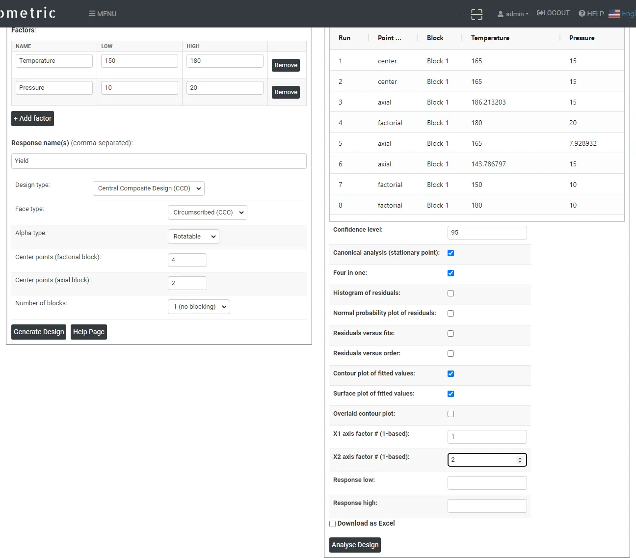
A process engineer wants to maximize the Yield of a chemical reaction, believed to depend on Temperature and Pressure in a curved (not purely linear) way, based on prior factorial experiments that showed significant curvature. A Central Composite Design (Circumscribed, Rotatable) is chosen for the two factors, Temperature (150–180°C) and Pressure (10–20 bar), with additional center points to test for lack-of-fit; the trials are run in random order and Yield is measured for each. The following steps were taken:

• Gathered the necessary data.
• Analysed the data with the help of https://statsai.zometric.com/ .
• To find Response Surface Design choose https://statsai.zometric.com/ > Statistical module > DOE > Create & Analyse Response Surface Design.
• Inside the tool, fed the data along with the design and analysis options as follows:

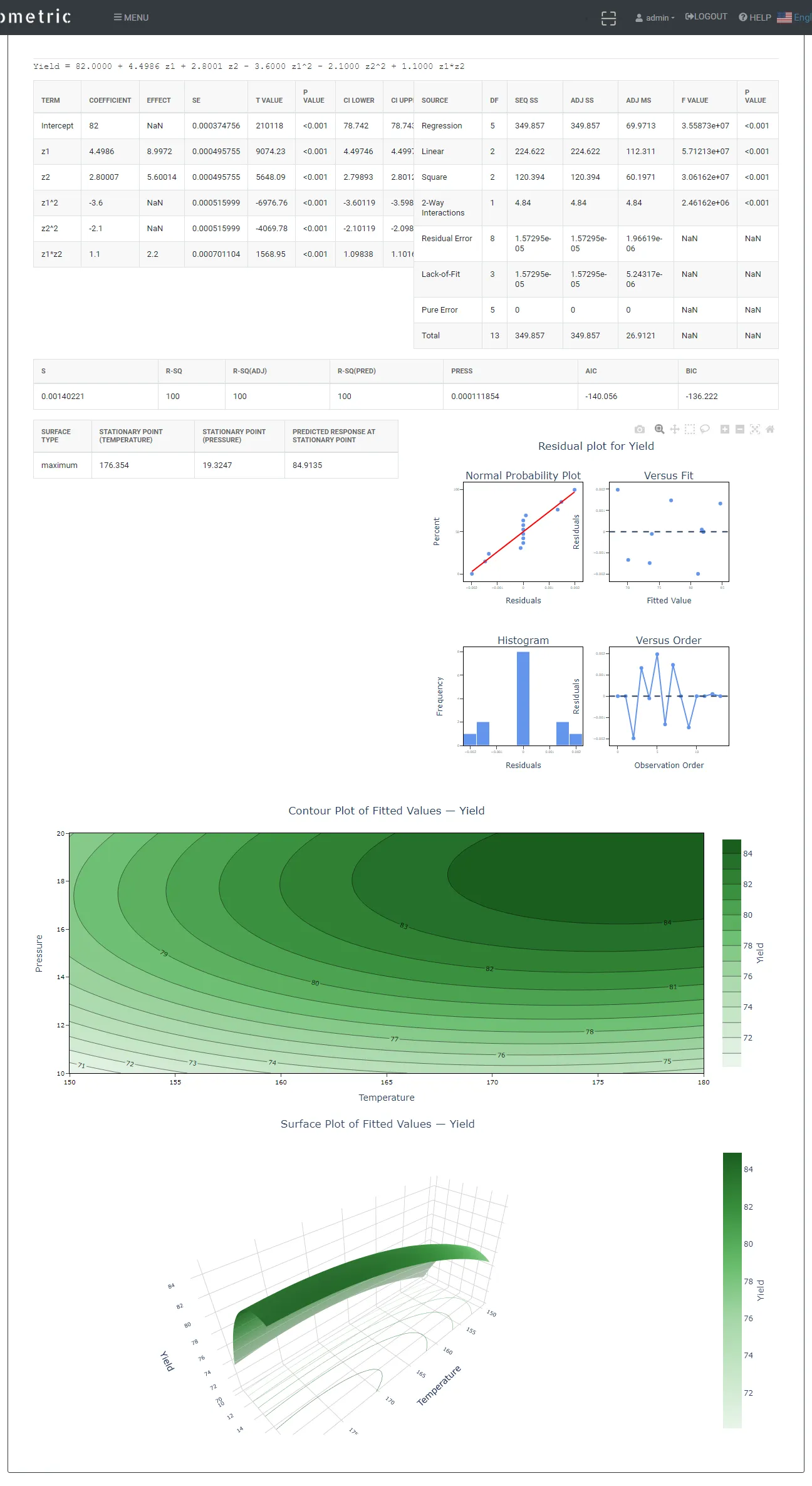
• After using the above mentioned tool, fetched the output as follows:

How to do Response Surface Design

The guide is as follows:

• Login in to Stats AI account with the help of https://statsai.zometric.com/
• On the home page, choose Statistical Tool > DOE > Create & Analyse Response Surface Design.
• Define your factors (name, low, high), choose a design type (CCD, Box-Behnken, or D-Optimal), and set its options.
• Click Generate Design, enter your measured Result(s) into the generated run matrix, choose analysis options, and click Analyse Design.
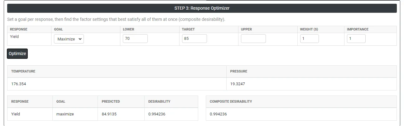
• Optionally, set a goal per response in Step 3 and click Optimize to find the best factor settings.

On the dashboard of Response Surface Design, the window is separated into two parts, with a third panel below for optimization.

On the left part, STEP 1: Define Factors & Generate Design is present.

• Factors: The continuous inputs you want to study (e.g. Temperature, Pressure). Enter a name, Low, and High value for each.
• Design type: Central Composite Design (CCD), Box-Behnken, or D-Optimal.
• Face type / Alpha type (CCD only): Controls the geometry of the axial points — Circumscribed, Inscribed, or Face-Centered, and whether the design is Rotatable or Orthogonal.
• Center points (CCD/Box-Behnken): How many replicated center-point runs to include, for lack-of-fit testing.
• Number of blocks (CCD only): Splits the design into 1, 2, or 3 blocks if the experiment must be run over multiple time periods or batches.
• Model type / Number of runs (D-Optimal only): The model (linear, interaction, or quadratic) the design should be optimized for, and how many runs you want.

On the right part, STEP 2: Enter Results & Analyse is present, along with the following options:

• Confidence level: The percent confidence used for the coefficient confidence intervals in the results table.
• Canonical analysis (stationary point): Reports the type of surface (maximum, minimum, saddle, or ridge) and the factor settings at its stationary point.
• Four in one / Histogram / Normal probability plot / Versus fits / Versus order: Residual diagnostic plots, to confirm the model fit is sound.
• Contour plot / Surface plot / Overlaid contour plot: Visualizes the fitted response surface across two chosen factors (specified by X1/X2 axis factor #), holding the others at their center value.
• Response low / Response high: For the overlaid contour plot — the acceptable response range to shade as feasible.
• Download as Excel: Exports the design, results, coefficients, and ANOVA to an Excel workbook.

Finally, STEP 3: Response Optimizer is present below, where you set a Goal (Maximize, Minimize, or Target), Lower, Target, Upper, Weight, and Importance per response, then click Optimize to find the factor settings that best satisfy all responses at once (composite desirability).