Multivariate Capability Index (MCpm)

Purpose

MCpm extends the familiar univariate Cpm capability index to two or more correlated quality characteristics measured jointly on the same part, treating them as ONE multivariate process rather than running separate univariate Cpk studies per characteristic (which double-counts shared variation and can materially mislead about true out-of-spec risk when the characteristics are correlated). It implements the index defined by Taam, Subbaiah & Liddy (1993, Journal of Applied Statistics), as precisely formalized by Santos-Fernandez & Scagliarini (2012, Journal of Statistical Software, in the MPCI R package documentation).

Key Capabilities

• Computes one joint capability index (MCpm) across 2 or more correlated variables, instead of separate univariate Cpk/Cpm values per variable.
• Accepts an independent LSL, USL and (optional) Target per variable, comma-separated in the same order as the selected Variables.
• Reports Cp (the joint spread-vs-tolerance ratio) and D (the off-target penalty factor) separately, so the two contributors to MCpm — process spread and how far off-center the process mean sits — can be diagnosed independently.
• Reports each variable's own semi-axis length in the modified tolerance region, giving a per-variable diagnostic alongside the single joint MCpm number.
• Configurable alpha (defaulting to the app-wide 0.0027 convention) controlling both the process's 99.73% probability region and, by analogy, the modified-tolerance-region convention.

Statistical Methods

MCpm is defined as a ratio of two ellipsoid volumes, corrected by an off-target penalty: MCpm = Cp / D, where Cp is the ratio of the volume of the largest axis-aligned ellipsoid inscribed in the rectangular specification region (R1) to the volume of the process's 99.73% probability ellipsoid (the region where a p-variate Normal process would place 1 − alpha of its mass, by default alpha = 0.0027), and D is a Mahalanobis-distance-based penalty for how far the process mean sits from target.

Region R1's semi-axes are simply a_i = min(USL_i − Target_i, Target_i − LSL_i) for each variable i — the largest axis-aligned ellipsoid that fits inside the rectangular tolerance box, independent of the process's own covariance structure. Its volume is Vol(R1) = (π^(p/2) / Γ(p/2 + 1)) · ∏ a_i.

The process's 99.73% probability ellipsoid (R3) is derived from the sample covariance matrix S: Vol(R3) = |S|^(1/2) · (πK)^(p/2) / Γ(p/2 + 1), where K is the (1 − alpha) quantile of the chi-square distribution with p degrees of freedom — the same distributional cutoff used to bound the process's own natural spread at the chosen confidence level.

Cp = Vol(R1) / Vol(R3) — how large the tolerance-region ellipsoid is relative to the process's own spread ellipsoid; Cp > 1 means the tolerance is comfortably larger than the process's natural spread.

D, the off-target penalty, is D = √(1 + (n / (n−1))·δ′ S⁻¹ δ), where δ = x̄ − Target is the vector of how far each variable's sample mean sits from its own target, and n is the sample size. D = 1 exactly when the sample mean equals the target vector, and grows as the process mean drifts off target (accounting for the correlation structure via S⁻¹, not just the raw per-variable offsets).

MCpm = Cp / D therefore equals 1 exactly when the process is centered on target and 99.73% of the process's probability mass falls inside the modified tolerance region; MCpm > 1 indicates a capable, reasonably-centered process, while MCpm < 1 indicates the process spread and/or off-target shift exceeds what the specification allows. This implementation was verified against Taam, Subbaiah & Liddy's own published worked example (25 parts, 2 variables), reproducing their reported MCpm = 1.825283 to full floating-point precision.

Input Fields & Options

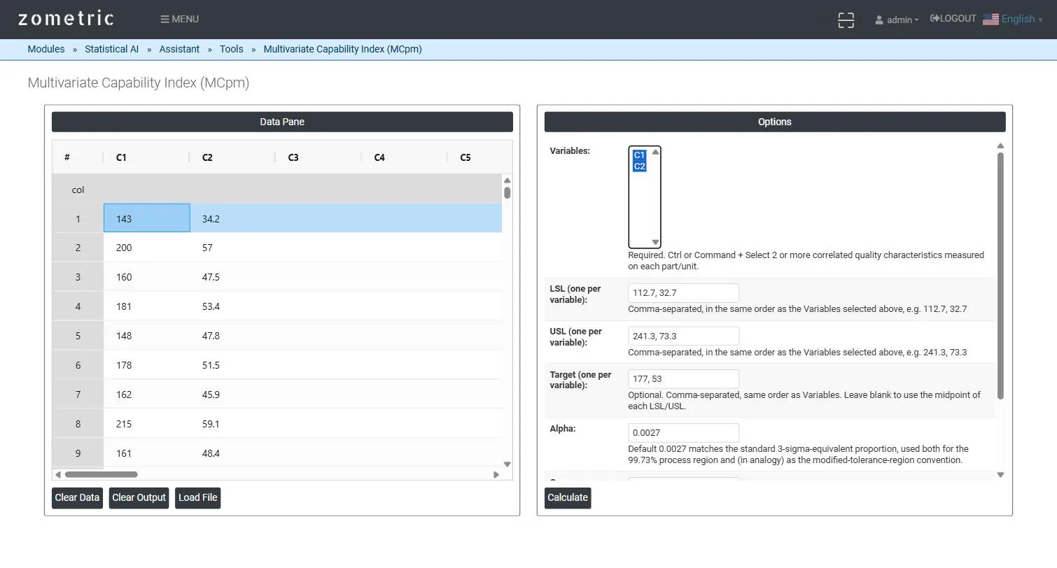
Figure 1 — 25 paired hardness/tensile-strength readings pasted into C1–C2, both selected as Variables, with per-variable LSL/USL/Target and Alpha = 0.0027.

Output Descriptions

• Summary table — Variables, p (number of variables), n (observations), Alpha, Cp (spread vs. modified tolerance), D (off-target penalty), and MCpm.
• Per-variable table — each variable's LSL, Target, USL, sample mean, and its semi-axis length a_i in the modified tolerance region.
• Plain-language interpretation — a one-paragraph explanation of what the computed MCpm value means for this process.
• PDF export via Download as PDF.

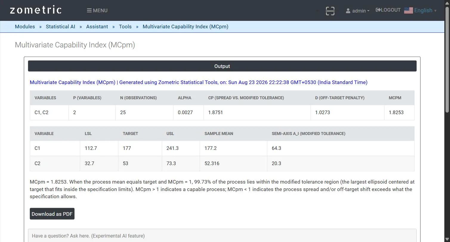
Figure 2 — MCpm output: the joint Cp/D/MCpm summary table and the per-variable LSL/Target/USL/Sample Mean/Semi-axis table.

Worked Example

A heat-treated steel part must simultaneously meet a hardness spec (C1, Brinell) and a tensile-strength spec (C2) that are physically correlated — harder parts tend to be stronger. Using the paper's own published 25-part worked example, with LSL = 112.7, 32.7, USL = 241.3, 73.3 and Target = 177, 53 for the two variables respectively, the tool reports Cp = 1.8751, D = 1.0273 and MCpm = 1.8253 — exactly matching Taam, Subbaiah & Liddy's own published result to full floating-point precision, confirming the process is capable and only slightly off-target once the correlation between hardness and tensile strength is properly accounted for.