Multiple Variables Process Capability

Purpose

Multiple Variables Process Capability answers a specific, common question that the app's existing capability tools could only answer indirectly: when the same characteristic is measured across several parallel variables — different cavities of an injection mold, different machines, different lines — against one shared specification, which one is worst? Rather than running N separate capability reports and comparing them by eye, this tool produces ONE unified side-by-side comparison table and one set of histograms, so every variable's Cp/Cpk-family indices sit in the same table.

Key Capabilities

• Select any 2 or more columns and get one aggregated comparison table instead of N stacked reports.
• A single LSL/USL pair is applied uniformly to every selected variable, so the comparison is always apples-to-apples against the same specification.
• Optional shared Target adds the Cpm index per variable to the same comparison table.
• Per-variable histograms with the shared spec limits overlaid, alongside the aggregated table.
• Configurable K-sigma tolerance multiplier, consistent with the app's other capability tools.

Statistical Methods

Each selected variable/column is treated as an independent process, run through the same Normal-capability engine used by the Automated Process Capability tool's Normal path. For each one, σ_overall is estimated via the moving-range method (MRbar/d2, or median-moving-range), and the standard z-based Performance index family is computed: Pp = (USL − LSL) / (K·σ), Ppu = (USL − x̄) / ((K/2)·σ), Ppl = (x̄ − LSL) / ((K/2)·σ), Ppk = min(Ppu, Ppl), with the default K = 6. Every variable always assumes Normality here — there is no per-variable normality test or nonnormal routing in this tool.

When a shared Target is supplied, Cpm is additionally computed per variable: Cpm = (USL − LSL) / (K·√(mean((x − Target)²))), penalizing a variable whose mean sits off-target even if its spread alone would otherwise look capable.

Because every variable is scored against the identical LSL/USL (and Target, when supplied), the resulting Ppk and Cpm values are directly comparable across variables — the variable with the lowest Ppk (or Cpm) in the comparison table is the worst-performing one relative to the shared spec.

PPM Expected is computed from the fitted Normal distribution's tail probability beyond each spec limit for that variable; PPM Observed is the empirical fraction of that variable's own sample falling outside the spec limits — letting a user spot cases where the two disagree (a sign the Normal-distribution assumption may not hold for that particular variable).

Input Fields & Options

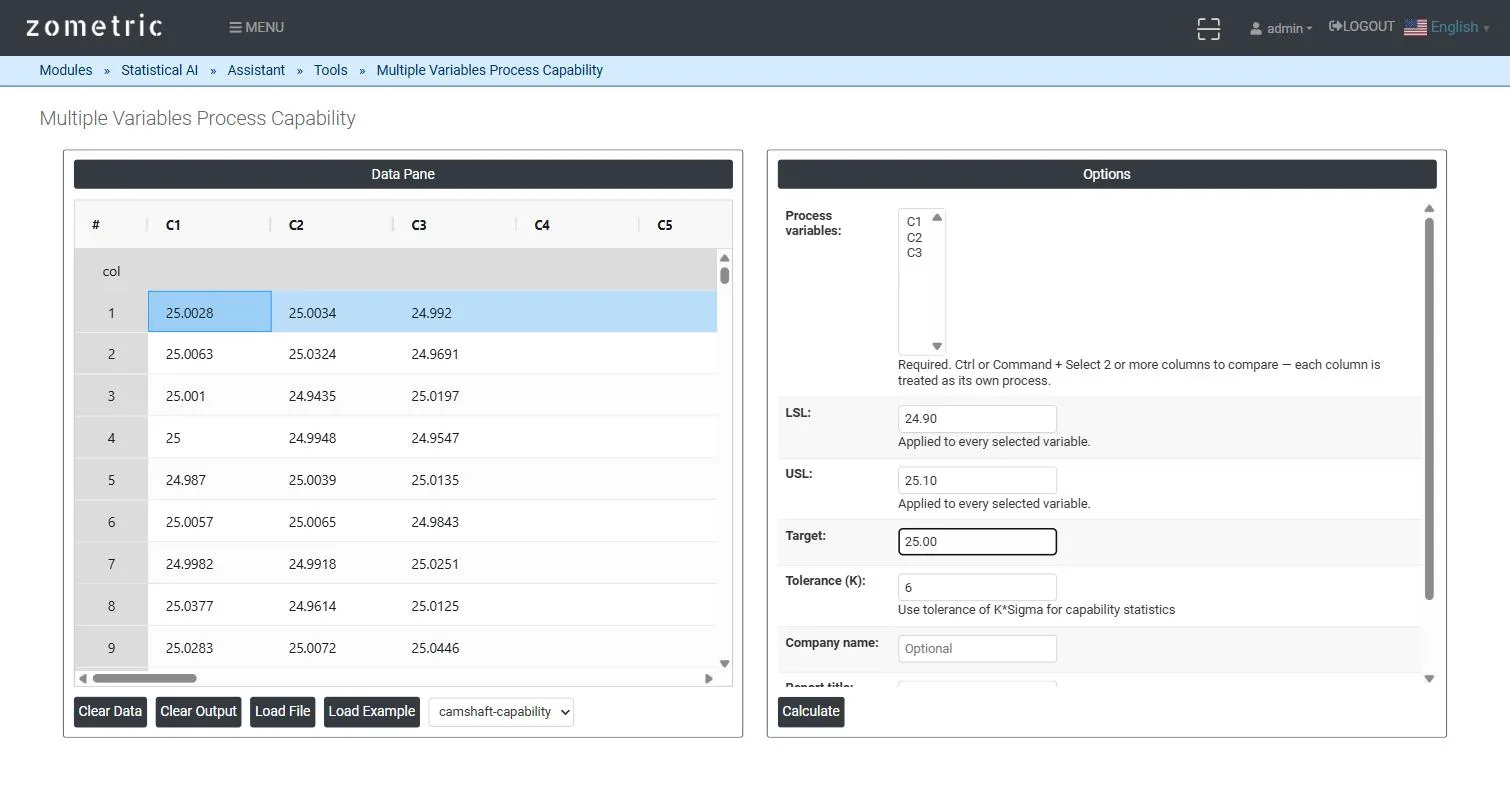
Figure 1 — Data pane with bore-diameter readings from 3 cavities in C1–C3, all three selected as Process variables, with a shared LSL/USL/Target.

Output Descriptions

• Comparison table — one row per selected variable with N, Mean, StDev, Pp, Ppl, Ppu, Ppk, Cpm (when Target is supplied), PPM Expected and PPM Observed, all against the same shared spec limits.
• Per-variable histogram — each variable's own distribution with the shared LSL/Target/USL reference lines and a fitted Normal curve.
• PDF export of the full comparison report via Download as PDF.

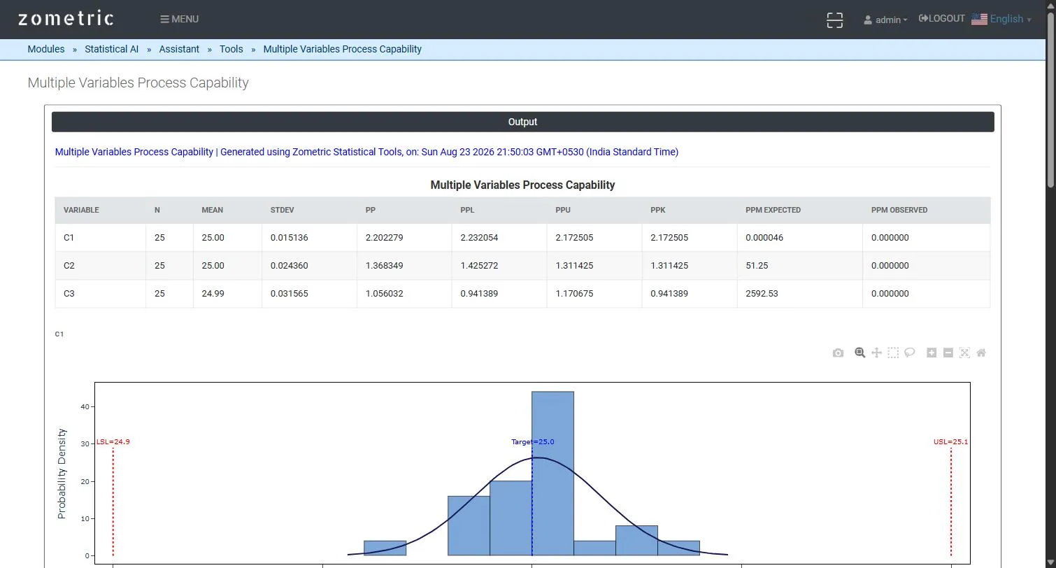
Figure 2 — The unified comparison table (N, Mean, StDev, Pp, Ppl, Ppu, Ppk, Cpm, PPM Expected, PPM Observed per variable) with the first variable's histogram.

Worked Example

An injection-molding tool has 3 cavities producing the same part; bore diameter (mm) is measured on 25 parts from each cavity (C1 = Cavity 1, C2 = Cavity 2, C3 = Cavity 3), against a shared LSL = 24.90, USL = 25.10, Target = 25.00. The comparison table shows Cavity 1 with the tightest spread (Ppk ≈ 2.17, Cpm ≈ 2.24) and Cavity 3 visibly worse (Ppk ≈ 0.94) — immediately flagging Cavity 3 as the one needing attention, without having to run and manually compare three separate reports.