
Accelerated Life Test Plan
On this page
Purpose
Accelerated Life Test Plan checks a proposed accelerated life test before you run it. You give your best assumptions about the product (Weibull shape and the characteristic life at two stress levels) and the plan you have in mind (test stress levels, how many units at each, total sample size and test duration). The tool reports how many failures to expect at each level and how precisely the test will estimate life at normal operating stress. Use it to compare plans and choose stress levels, sample sizes and test length before committing units and chamber time.
Key Capabilities
- Arrhenius, Inverse Power Law or Linear life-stress relationship, with a Weibull life distribution.
- Expected number and percentage of failures at each test stress by the end of the test.
- Precision of the estimated life at use stress from repeated simulated tests: the standard error of log(life) and a multiplicative confidence factor.
- Any number of test stress levels with your own allocation of units.
- No data needed: everything is entered as planning assumptions.
Statistical Methods
The assumed life-stress line is set by two points: the characteristic life (Weibull scale η, the time by which 63.2% fail) at the use stress and at an anchor stress. The relationship transforms stress S as 1/S for Arrhenius (S in kelvin), ln(S) for Inverse Power Law and S for Linear, and the model is ln(η) = a + b · g(S), so a and b follow from the two points. From this line the tool computes η at each test stress. The units at each level are the total sample size times the allocation fraction, rounded, with the last level taking any rounding difference.
With a test of fixed duration T (units still running at T are censored), the probability that a unit fails during the test at a stress with scale η is 1 − exp(−(T/η)^β), where β is the assumed shape. The expected failures at a level are this probability times the number of units there.
Precision is estimated by Monte Carlo simulation: the tool simulates 150 complete tests from the assumed model with the planned allocation and censoring, fits each simulated data set with a Weibull regression (common shape, ln(η) linear in the transformed stress, by maximum likelihood) and records the estimated log characteristic life at use stress. The standard deviation of these estimates is the SE of log(life). The precision factor is exp(−z·SE) to exp(z·SE), where z is the standard normal value for the confidence level: the estimate from a real test is expected to lie within these multiples of the true life. A fixed random seed is used, so the same inputs give the same result. Results depend on the assumptions, especially the shape, so try a range of plausible values.
Input Fields & Options
Field | Description |
Life-stress relationship | Arrhenius (stress = temperature in Kelvin) (default), Inverse Power Law or Linear. |
Assumed Weibull shape | Required. From prior data or engineering judgement; the plan's precision estimate depends on this assumption. |
Use (normal-operating) stress level | Required. The stress at which you want to estimate life, e.g. 323 K. |
Assumed characteristic life at use stress | Required. Your best estimate of the Weibull scale at use stress. |
A second (anchor) stress level | Required. Typically a high stress you have prior data or an engineering estimate for; with its life, it fixes the assumed life-stress line. |
Assumed characteristic life at that anchor stress | Required. The Weibull scale at the anchor stress. |
Candidate test stress levels | Required. Space or comma-separated, e.g. 333 353 373: the stress levels the plan will test at. |
Allocation fractions | Required. Space or comma-separated, same count and order as the stress levels, summing to 1, e.g. 0.4 0.3 0.3: the fraction of the total sample tested at each level. |
Total sample size | Required. At least 4. |
Planned test duration (censoring time) | Required. Units still running at this time are censored. |
Confidence level (%) | For the precision factor. Default 95; 50 to 99.99. |
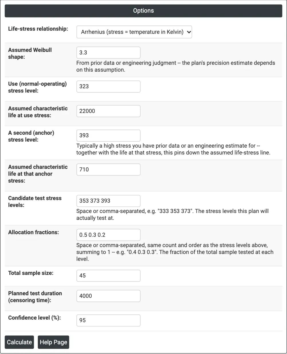
Figure 1 — Options for the capacitor test plan: Arrhenius, shape 3.3, 22,000 h at 323 K and 710 h at 393 K, 45 units split 0.5/0.3/0.2 over 353, 373 and 393 K, 4,000-hour test.
Output Descriptions
- Plan summary — Assumed Shape (Weibull), Assumed Life at Use Stress, Total Sample Size, Total Expected Failures, Simulations Used, Failed Fits, SE of log(Life) at Use Stress and the Precision Factor on Life at Use Stress (multiply/divide by) at the chosen confidence level.
- Per-level table — Stress Level, N, Assumed Scale (at this stress), Expected Failures by Censor Time and Expected %Failing.
- PDF export via Download.
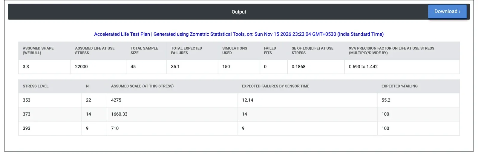
Figure 2 — Plan results: 35.1 expected failures out of 45 units, SE of log(life) 0.1868, and a 95% precision factor of 0.693 to 1.442 on life at 323 K.
Worked Example
A reliability engineer plans a temperature test for an electrolytic capacitor that runs at 323 K. From an earlier test the engineer expects a Weibull shape of about 3.3, a characteristic life of about 22,000 hours at 323 K and 710 hours at 393 K. The engineer proposes 45 capacitors at 353, 373 and 393 K, with half of them at the lowest temperature (fractions 0.5, 0.3, 0.2), and a test length of 4,000 hours.
The plan puts 22, 14 and 9 units at the three temperatures. The assumed characteristic life is 4,275 hours at 353 K, 1,660 hours at 373 K and 710 hours at 393 K, so 55.2% of the 353 K units (12.1 of 22) are expected to fail within 4,000 hours, and essentially all units at 373 and 393 K. In total 35.1 failures are expected. Over 150 simulated tests the SE of log(life) at 323 K is 0.1868, and the 95% precision factor is 0.693 to 1.442: the estimated life at 323 K from this test is likely to fall between about 0.69 and 1.44 times the true value.
Changing the plan shows where precision comes from. Doubling the sample to 90 units narrows the factor to 0.772 to 1.296, and extending the test to 8,000 hours narrows it to 0.752 to 1.329. An equal split of units (0.34, 0.33, 0.33) gives slightly wider limits, 0.685 to 1.460, with fewer units at the temperature closest to use. Moving the lowest level down to 343 K gives only 26.0 expected failures and a wider factor of 0.605 to 1.653. If the true shape is 2 rather than 3.3, the factor widens to 0.547 to 1.827, so a pessimistic shape is worth checking before the plan is fixed.