
Accelerated Life Testing
On this page
Purpose
Accelerated Life Testing analyses life data from a test run at raised stress levels (temperature, voltage, load) and uses a life-stress relationship to estimate life at normal operating stress. Products often last too long at normal conditions to test directly, so units are run hotter or harder to make them fail sooner. The tool fits one Weibull model to all the data, in which the characteristic life depends on stress through the chosen relationship and the shape is common to all stress levels, and extrapolates to the use stress.
Key Capabilities
- One Weibull maximum-likelihood fit to all stress levels together, with right-censored units (still running at the end of the test).
- Three life-stress relationships: Arrhenius (temperature in kelvin), Inverse Power Law and Linear.
- Intercept, slope and common shape with standard errors, Z tests and confidence intervals, and the log-likelihood.
- Separate Weibull fits at each stress level, to check the common-shape assumption.
- Estimated 10th, 50th and 90th percentile life at a use stress you enter, with confidence intervals.
- Life-stress plot of ln(characteristic life) against the transformed stress, with the fitted line and its confidence band.
Statistical Methods
The model is ln(η) = a + b · g(S), where η is the Weibull scale (characteristic life, the time by which 63.2% fail) at stress S, and the shape β is the same at every stress. The relationship sets g: Arrhenius uses g = 11604.83 / S with S in kelvin, so b is the activation energy in electronvolts (11604.83 is 1 / Boltzmann's constant in K/eV); Inverse Power Law uses g = ln(S); Linear uses g = S. a, b and β are estimated together by maximum likelihood over all units, a failure contributing its Weibull density and a censored unit its survival probability, as in Minitab. Standard errors come from the inverse of the numerical Hessian of the log-likelihood; Z = estimate / SE with a two-sided normal p-value, and the confidence intervals are estimate ± z × SE, on the log scale for the shape.
The acceleration factor between two temperatures T₁ < T₂ is exp(b × 11604.83 × (1/T₁ − 1/T₂)) for Arrhenius. For Inverse Power Law, life is proportional to S^b, so a negative slope means life falls as stress rises. The tool also fits a separate Weibull distribution at each stress level and lists its scale and shape: these are only a check that the shapes are similar, as the model assumes the same failure mechanism at every level; they are drawn as points on the life-stress plot.
At the use stress, the life by which p% fail is t_p = exp(a + b · g(S_use) + ln(−ln(1 − p/100)) / β). Its confidence interval is formed on ln(t_p) with the delta method from the covariance matrix of a, b and β, and converted back with exp, so it is not symmetric. The band on the life-stress plot is the confidence interval for a + b · g. Estimates at a use stress outside the tested range are extrapolations and depend on the relationship holding there.
Input Fields & Options
Field | Description |
Time variable | Required. Time to failure, or time to censoring for units still running. |
Use censoring column | Required. Rows equal to the censoring value are right-censored; every other row is a failure. |
Censoring value | The value in the censoring column that marks a unit still running when the test stopped. Default 0, so 1 = failure. |
Stress variable | Required. The test stress of each unit. Needs at least 2 distinct stress levels, with enough failures at each to fit a Weibull distribution. |
Life-stress relationship | Arrhenius (stress = temperature in Kelvin) (default), Inverse Power Law, or Linear. |
Use (normal-operating) stress level | Optional. If given, the tool estimates life percentiles at this stress, in the same units as the stress variable. |
Confidence level (%) | Default 95; 50 to 99.99. Sets the confidence intervals for the intercept, slope and shape, for the lives at the use stress, and the band on the life-stress plot. |
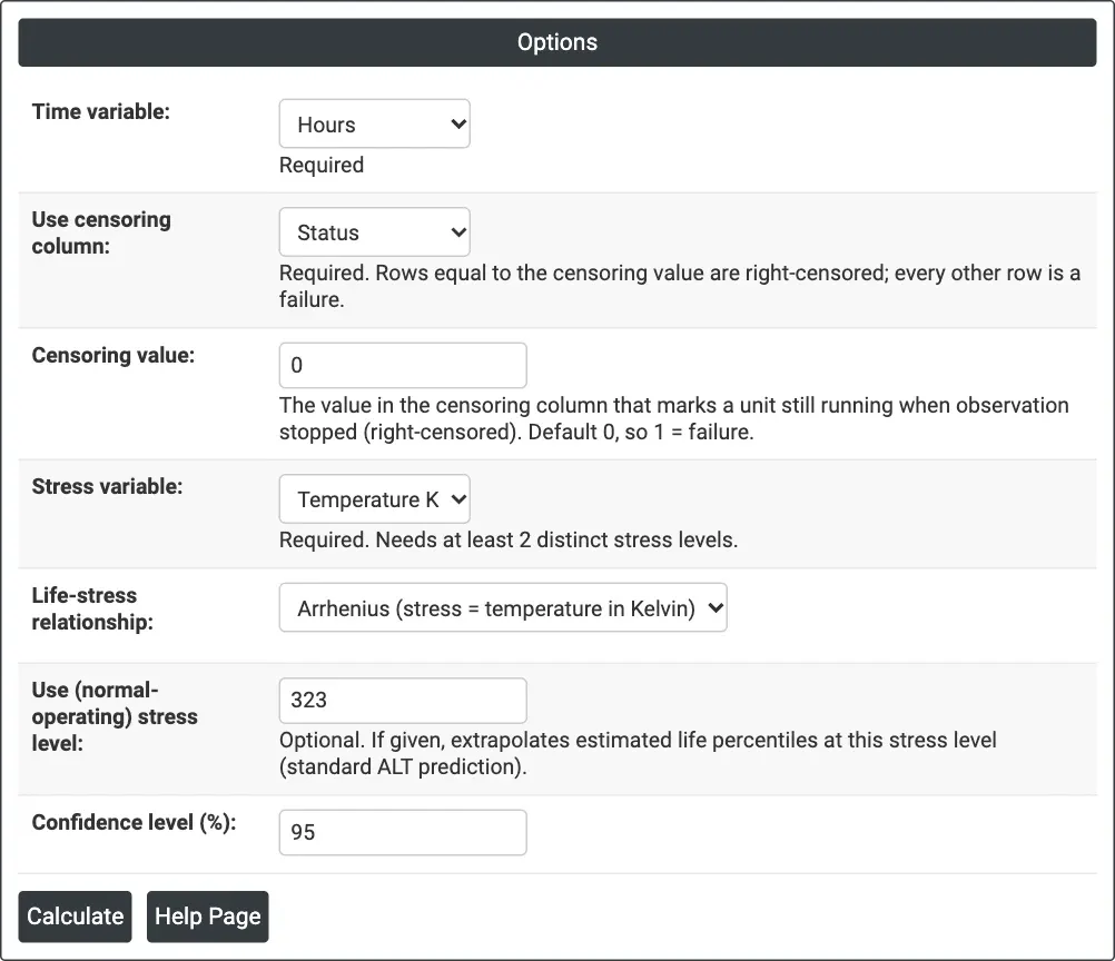
Figure 1 — Options for the capacitor example: hours to failure, Status as the censoring column, temperature in kelvin as the stress, Arrhenius relationship, use stress 323 K.
Output Descriptions
- Method — distribution (Weibull), relationship, Shape (common), Log-Likelihood and number of stress levels.
- Per-level fits — stress level, N, Weibull scale and shape from a separate fit at each level.
- Life-stress relationship — Intercept (a), Slope (b) and Shape with SE, Z, P and confidence limits.
- Estimated life at use stress — shown when a use stress is entered: the life by which 10%, 50% and 90% of units fail, with confidence limits.
- Life-Stress Relationship plot — ln(Scale) against the transformed stress (11604.83 / Temperature (K), ln(Stress) or Stress), with the per-level fits as points, the fitted line and its confidence band (dotted).
- PDF export via Download.
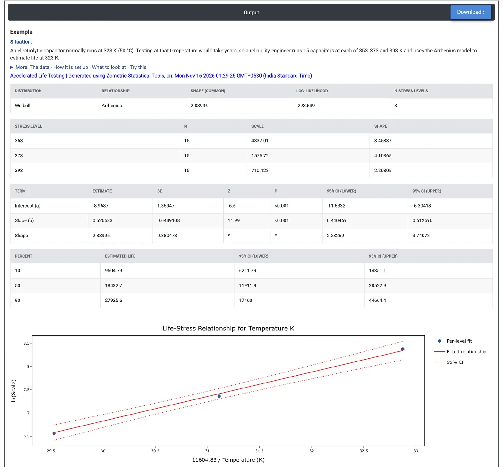
Figure 2 — Capacitor results: common shape 2.89, Arrhenius slope 0.527 eV, and a median life of 18,433 h at 323 K (95% CI 11,912 to 28,523 h).
Worked Example
An electrolytic capacitor normally runs at 323 K (50 °C). Testing at that temperature would take years, so a reliability engineer runs 15 capacitors at each of 353, 373 and 393 K. At 353 K the test stops at 4,000 hours, when 8 of the 15 have failed; at 373 and 393 K all 15 fail. The engineer sets Time variable = Hours, Use censoring column = Status (Censoring value 0), Stress variable = Temperature K, Life-stress relationship = Arrhenius and Use (normal-operating) stress level = 323.
The common shape is 2.890 (95% CI 2.233 to 3.741): wear-out failures. The slope is 0.5265 (SE 0.0439, Z = 11.99, p < 0.001, 95% CI 0.4405 to 0.6126), so the activation energy is about 0.53 eV and temperature clearly shortens life. On the fitted model, life at 353 K is 2.5 times that at 373 K, and life at 323 K is 5.0 times that at 353 K. The separate fits give characteristic lives of 4,337, 1,576 and 710 hours and shapes of 3.46, 4.10 and 2.21 at 353, 373 and 393 K; the shapes scatter around the common value; a level whose shape stood far apart from the others would suggest a different failure mechanism there.
At 323 K, 10% of capacitors are expected to fail by 9,605 hours (95% CI 6,212 to 14,851), half by 18,433 hours (11,912 to 28,523) and 90% by 27,926 hours (17,460 to 44,664). These numbers match Minitab's Accelerated Life Testing on the same data. They are extrapolations below the lowest test temperature, which is why the intervals are wide, and hold only if the same failure mechanism acts at 323 K. As a check, setting the use stress to 353 K gives 10% failing by 1,924 hours and half by 3,693 hours, in line with 8 of 15 failing within 4,000 hours in the 353 K test. The Inverse Power Law relationship gives a median of 15,643 hours at 323 K, so the choice of model changes the extrapolation by about 15%; for temperature, Arrhenius is the usual choice.