
Analysis of Means (ANOM)
On this page
Purpose
Analysis of Means (ANOM) compares the mean of each group with the overall mean and shows, on a chart like a control chart, which groups are significantly above or below it. Use it to compare suppliers, machines, shifts or operators when the question is which ones are out of line, not just whether some difference exists. It also handles defectives (binomial) and defect counts (Poisson) per sample.
Key Capabilities
- Normal data: one factor, or two factors with interaction and main-effect charts (balanced designs).
- Binomial data: proportion defective in samples of equal size.
- Poisson data: defect counts per sample.
- ANOM chart with the centre line, upper and lower decision limits and the out-of-limit groups marked.
- Table of each group's mean, limits, signal and p-value.
- Data Options: subset the rows before the analysis.
Statistical Methods
For normal data with one factor, the centre line is the grand mean of all observations and s is the pooled standard deviation of the groups, with N − k degrees of freedom for N observations in k groups. The decision limits for group i are grand mean ± h·s·√((N − nᵢ) / (N·nᵢ)). A group whose mean lies outside its limits differs significantly from the overall mean. The critical value h controls the overall risk α of any false signal: for two groups it is the t value t(1 − α/2); for a balanced design with α from 0.001 to 0.1 it is the exact ANOM value (the upper α point of the largest of k correlated t statistics, found by simulation); otherwise a Sidak-type t value. Each group's p-value comes from the same distribution.
With two factors (balanced data only), the error mean square comes from the full two-way ANOVA. The interaction chart plots the cell effects (cell mean − row mean − column mean + grand mean) around zero, and the main-effect charts plot each factor's level means around the grand mean, each with its own decision limits. Look at the interaction chart first: if it signals, the main effects must be read with care.
For binomial data each row is the number of defectives in a sample of size n; the points are pᵢ = yᵢ / n, the centre line is p̄, s = √(p̄(1 − p̄)/n), and the limits are p̄ ± h·s·√((k − 1)/k) with h = z(1 − α/(2k)) (z(1 − α/2) for two samples). For Poisson data each row is a count; the centre line is c̄ and s = √c̄. ANOM for normal data assumes normal errors with equal variances in the groups.
Input Fields & Options
Field | Description |
Response | Numeric column. For Binomial or Poisson: one count per sample (row). Required. |
Distribution of data | Normal (default), Binomial or Poisson. |
Factor 1 | Grouping column. Required for Normal data. |
Factor 2 (optional) | Second factor for a two-way ANOM: interaction and main effects (balanced designs). |
Sample size | Shown for Binomial: the number of items in each sample. |
Alpha level | Overall risk of a false signal; default 0.05, from 0.001 to 0.5. |
Data Options: Subset (optional) | Exclude matching rows (default) or Include only matching rows, by row numbers and/or a condition. |
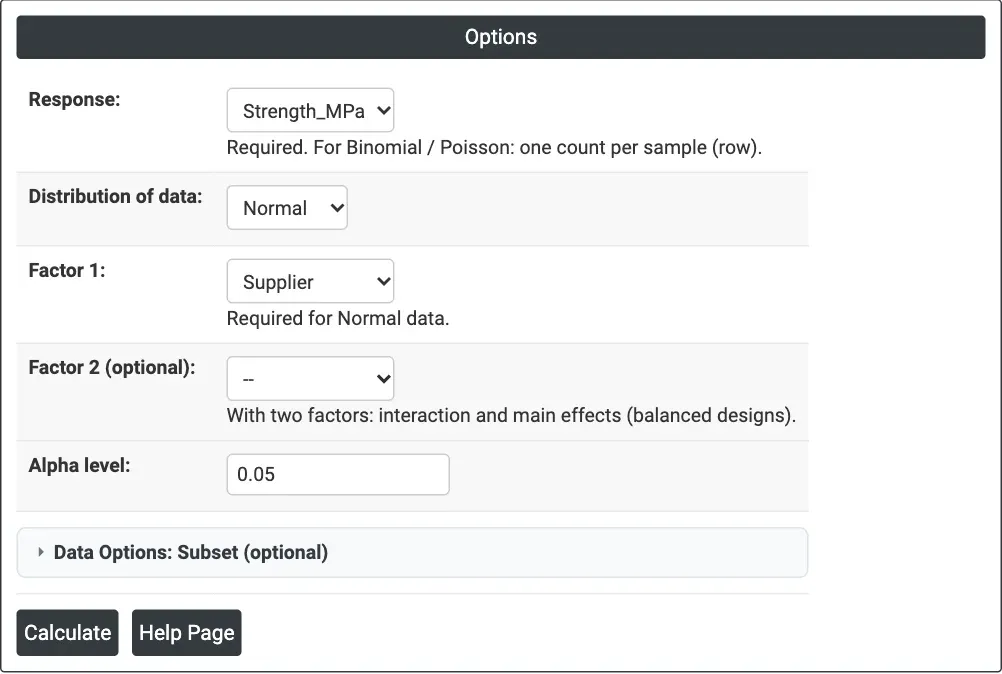
Figure 1 — Options for the supplier example: Strength_MPa by Supplier, normal data, alpha 0.05.
Output Descriptions
- ANOM chart — group means (or proportions or counts) with the centre line and the upper (UDL) and lower (LDL) decision limits; points outside are marked in red.
- Method — hypotheses, alpha, number of groups, error degrees of freedom and the critical value h (for two factors: the design and MSE).
- Analysis of Means — N, Mean, Center Line, LDL, UDL, Signal and P-Value for each group (for two factors: tables of interaction effects and of each factor's main effects).
- PDF export via Download.
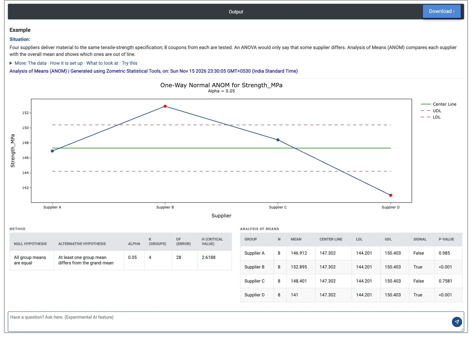
Figure 2 — One-way ANOM of coupon strength by supplier: Supplier B is above the upper decision limit and Supplier D below the lower one.
Worked Example
Four suppliers deliver material to the same tensile-strength specification. The quality engineer tests 8 coupons from each supplier and wants to know which suppliers differ from the average. The engineer selects Strength_MPa as the response, Supplier as Factor 1, normal data and alpha 0.05.
The centre line is 147.30 MPa and, with 28 error degrees of freedom and h = 2.6188, the decision limits are 144.20 to 150.40 MPa (pooled standard deviation about 3.87 MPa). Supplier B averages 152.90 MPa, above the upper limit, and Supplier D 141.00 MPa, below the lower limit: both signal with p < 0.001. Suppliers A (146.91, p = 0.985) and C (148.40, p = 0.7581) cannot be told apart from the average.
At alpha 0.01 the limits widen to 143.39 to 151.21 MPa, and B and D are still outside. The engineer raises a supplier corrective action with D, whose coupons are about 6 MPa weaker than the average, and checks whether B's process can be used as the reference.