
ARIMA (Box-Jenkins Forecasting)
On this page
Purpose
ARIMA fits a Box-Jenkins autoregressive integrated moving average model to a series measured at equal time intervals (daily, weekly, monthly) and forecasts the next values with prediction intervals. Use it when each value depends on the values before it, or when the series has a trend or a repeating season that simpler methods such as moving averages or exponential smoothing do not capture well. The autocorrelation (ACF) and partial autocorrelation (PACF) plots of the series help choose the model orders before you run it.
Key Capabilities
- Non-seasonal autoregressive (p), differencing (d) and moving average (q) terms, plus seasonal terms (P, D, Q) for any seasonal period, e.g. 12 for monthly data with a yearly pattern or 7 for daily data with a weekly pattern.
- Optional constant term: the mean level of an undifferenced series, or the average drift (trend) of a differenced one.
- Parameter estimates with standard errors, T-values and p-values, so you can drop terms that are not needed.
- Residual checks: residual sum of squares and mean square, Modified Box-Pierce (Ljung-Box) chi-square tests at lags 12, 24, 36 and 48, and ACF and PACF plots of the residuals.
- Forecasts with lower and upper prediction limits at the confidence level you choose; a forecast origin lets you forecast from an earlier row and compare the forecasts with what actually happened.
- Fit accuracy measures MAPE, MAD and MSD, comparable with the other time series tools.
- Optional extra output: estimates at each iteration, the correlation matrix of the estimated parameters, the back forecasts, and a four-in-one residual plot.
Statistical Methods
The model is φ(B)Φ(Bˢ)(1−B)ᵈ(1−Bˢ)ᴰ yₜ = C + θ(B)Θ(Bˢ) aₜ, where B is the backshift operator, φ and θ are the non-seasonal AR and MA polynomials of orders p and q, Φ and Θ are the seasonal AR and MA polynomials of orders P and Q in Bˢ, s is the seasonal period, C is the constant and aₜ are the residuals (random shocks). The differencing (1−B)ᵈ(1−Bˢ)ᴰ removes trend and season before the AR and MA terms are fitted, so d + D·s observations are lost at the start of the series.
The parameters are estimated by the Box-Jenkins least squares method with back forecasts: starting values are refined iteratively to minimise the sum of squared residuals, with the series forecast backwards to provide its pre-sample values. The residual mean square MS = SS / DF, with DF = number of differenced observations − number of estimated parameters. Each coefficient’s T-value is the coefficient divided by its standard error, with the p-value from the t distribution on the residual DF. For an undifferenced model with a constant, the process mean C / (φ(1)Φ(1)) is also reported.
The Ljung-Box statistic Q = n(n+2) Σ rₖ² / (n−k) is computed from the residual autocorrelations rₖ up to each lag and compared with a chi-square distribution whose DF is the lag minus the number of estimated parameters; a p-value above 0.05 means no evidence that autocorrelation is left in the residuals. Forecasts are made recursively from the fitted equation; the prediction interval for h periods ahead is the forecast ± z·√(MS·Σψⱼ²), summing the first h ψ weights of the model, so the intervals widen with the forecast horizon.
Input Fields & Options
Field | Description |
Variable (Y) | Required. The column holding the series, in time order, at equal intervals. |
Autoregressive order (p) | Number of non-seasonal AR terms (0 to 10, default 1): how many previous values carry over into the current one. |
Difference order (d) | Number of non-seasonal differences (0 to 3, default 0). Use 1 for a series with a trend that wanders or grows. |
Moving average order (q) | Number of non-seasonal MA terms (0 to 10, default 0): how many previous random shocks carry over. |
Include seasonal terms | Tick to add the seasonal orders below. The model needs at least one AR or MA term in total. |
Seasonal AR order (P) / Seasonal difference order (D) / Seasonal MA order (Q) | Seasonal orders (P and Q 0 to 5, D 0 to 2). D = 1 models the year-on-year change for monthly data with s = 12. |
Seasonal period (s) | Required with seasonal terms: the number of observations in one season (12 for monthly data with a yearly cycle, 4 for quarterly, 7 for daily data with a weekly cycle). |
Include constant term | Ticked by default. Untick it for a differenced series with no drift. |
Number of forecasts | How many periods to forecast after the forecast origin (0 to 1000; 0 = no forecasts). |
Confidence level (%) for forecast interval | Default 95. |
Forecast origin (row) | Optional. Forecasts start after this row, using the data up to it; blank = end of the series. Use it to test the model against data you already have. |
Results to display | Final estimates, differencing information, residual sums of squares, number of observations; or in addition the estimates at each iteration, the correlation matrix of the estimated parameters, or the back forecasts. |
Residual plots (four in one) | Adds a normal probability plot, residuals versus fits, a histogram and residuals versus order. |
Title | Title shown on the output. |
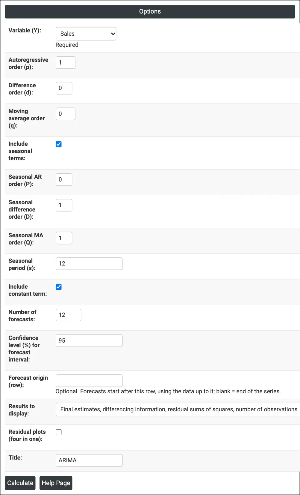
Figure 1 — The monthly sales example: Variable (Y) = Sales, a seasonal ARIMA(1, 0, 0)(0, 1, 1)12 model with a constant and 12 forecasts.
Output Descriptions
- ARIMA plot — the series with the fitted values, the forecasts and their prediction interval band; MAPE, MAD and MSD are shown under the title.
- Final Estimates of Parameters — each AR, SAR, MA and SMA term and the constant, with coefficient, SE Coef, T-Value and P-Value (and the Mean for an undifferenced model with a constant).
- Residual Sums of Squares — DF, SS and MS of the residuals.
- Modified Box-Pierce (Ljung-Box) Chi-Square statistic — Chi-Square, DF and P-Value at lags 12, 24, 36 and 48 (lags longer than the series are left out).
- Forecasts — period, forecast, and lower and upper prediction limits.
- ACF and PACF of Residuals — bars inside the dashed limits mean no autocorrelation is left.
- Optional tables and plots chosen in Results to display and Residual plots, and PDF export via Download.
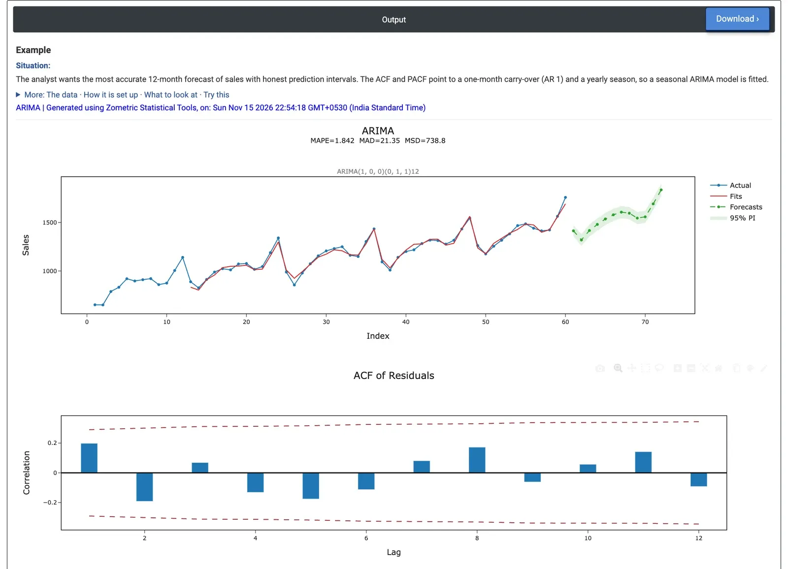
Figure 2 — ARIMA output for the monthly sales example: the fit and 12-month forecast with its 95% prediction band, and the ACF of the residuals.
Worked Example
An analyst has 60 months of sales (January 2020 to December 2024) and wants a 12-month forecast with honest prediction intervals. The ACF and PACF point to a one-month carry-over and a yearly season, so the model is ARIMA(1, 0, 0)(0, 1, 1)12 with a constant: Autoregressive order (p) = 1, Seasonal difference order (D) = 1, Seasonal MA order (Q) = 1, Seasonal period (s) = 12, and Number of forecasts = 12.
Both terms are clearly needed: AR 1 = 0.481 (SE 0.104, T = 4.63, p < 0.001) and SMA 12 = 0.805 (SE 0.144, T = 5.59, p < 0.001), with a constant of 69.34 (the average year-on-year growth). The residual MS is 788.1 on 45 DF (60 months − 12 lost to the seasonal difference − 3 parameters). The Ljung-Box p-values are 0.214, 0.319 and 0.254 at lags 12, 24 and 36, all above 0.05, so the residuals look like random noise and the model has captured the pattern. The fit is close: MAPE 1.84%, MAD 21.35, MSD 738.8.
The forecast for January 2025 (period 61) is 1,414 units with a 95% prediction interval of 1,359 to 1,469, rising to 1,837 for December 2025 (period 72), interval 1,774 to 1,899. To test the model before trusting it, set Forecast origin (row) = 48 to forecast 2024 from the data up to December 2023 and compare the forecasts with the actual 2024 sales.