
Augmented Dickey-Fuller Test
On this page
Purpose
The Augmented Dickey-Fuller (ADF) test checks whether a time series is stationary, that is, whether it varies around a fixed mean (or a fixed trend) or wanders without returning. Many forecasting models, ARIMA in particular, assume a stationary series. Run the test before fitting such a model to decide whether to model the raw data, model a trend, or difference the series first.
Key Capabilities
- Tests the null hypothesis of a unit root (non-stationary series) against a stationary alternative.
- Four forms of the test regression: around a constant, a constant and linear trend, a constant with linear and quadratic trend, or with neither.
- Chooses the number of lagged differences automatically by AIC, BIC or the t-statistic of the last lag, or uses a fixed number you enter.
- Reports the test statistic, p-value, lags used and the 1%, 5% and 10% critical values, with a plain-language conclusion at your significance level.
Statistical Methods
The test fits the regression Δyₜ = α + βt + γ·yₜ₋₁ + δ₁Δyₜ₋₁ + … + δₖΔyₜ₋ₖ + εₜ, where Δyₜ = yₜ − yₜ₋₁. The constant α and trend βt are included or left out according to Regression type (the quadratic option adds a t² term). The test statistic is the t-ratio of γ. If the series has a unit root, γ = 0; a strongly negative statistic means the series is pulled back towards its mean or trend, so it is stationary. The statistic does not follow the usual t distribution: the p-value uses MacKinnon's approximate distribution and the critical values come from MacKinnon's tables, both for the regression type chosen.
The lagged differences Δyₜ₋ᵢ absorb short-term autocorrelation. Maximum lag defaults to min(n/2 − 3, 12·(n/100)^¼), rounded down. With AIC or BIC the tool fits every lag from 0 to the maximum and keeps the one with the lowest criterion; with t-stat it starts at the maximum and drops lags until the last lag has |t| ≥ 1.645; with Fixed it uses the maximum lag exactly. N Observations is the number of rows left in the regression: n − lags used − 1. The calculation uses statsmodels' adfuller. The series must have no gaps and at least 6 values.
If the p-value is below the significance level, the null hypothesis of a unit root is rejected and the series is treated as stationary; otherwise it is likely non-stationary and differencing (or a trend term) is needed. The significance level only changes this conclusion line; the critical values are always shown at 1%, 5% and 10%.
Input Fields & Options
Field | Description |
Variable | Required. The numeric column holding the series, in time order. |
Regression type | Constant (test for stationarity around a mean), the default; Constant and trend (test for stationarity around a trend); Constant, linear, and quadratic trend; or None (no constant, no trend). |
Lag selection method | AIC (minimize Akaike Information Criterion), the default; BIC (minimize Bayesian Information Criterion); t-stat (drop lags while the last lag's t-stat is insignificant); or Fixed (use Maximum lag exactly). |
Maximum lag | Optional. Upper limit searched by AIC, BIC and t-stat, or the exact lag used with Fixed. Blank uses min(n/2 − 3, 12·(n/100)^¼). |
Significance level | Default 0.05 (0.001 to 0.5). The p-value is compared with it for the conclusion. |
Title | Title shown on the output. |
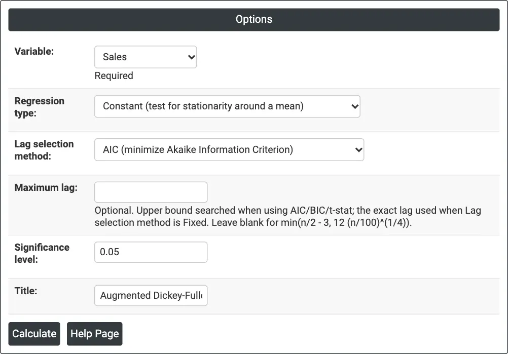
Figure 1 — Testing monthly Sales with a constant only, lags chosen by AIC, at a 0.05 significance level.
Output Descriptions
- Test — the variable, test statistic, p-value, number of lagged differences used, the maximum lag searched and the number of observations in the test regression.
- Critical Values — the critical values of the test statistic at 1%, 5% and 10% for the chosen regression type. The series is stationary at a level if the statistic is below (more negative than) its critical value.
- Conclusion — a sentence that compares the p-value with the significance level and says whether the series is likely stationary or non-stationary.
- PDF export via Download.
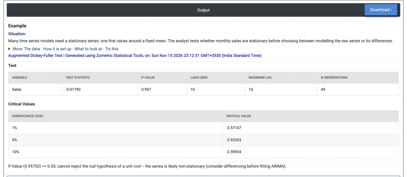
Figure 2 — Monthly sales tested around a fixed mean: statistic −0.018, p-value 0.957, so the series is not stationary.
Worked Example
A sales analyst at a consumer electronics distributor has 60 months of unit sales (January 2020 to December 2024) and plans an ARIMA forecast. First the analyst tests whether the sales are stationary. The analyst selects Variable = Sales and keeps Regression type = Constant, Lag selection method = AIC and Significance level = 0.05.
The maximum lag searched is 10 and AIC keeps all 10, leaving 49 observations in the test regression. The test statistic is −0.018 with a p-value of 0.957; the 5% critical value is −2.92 and the statistic is nowhere near it. The unit root cannot be rejected: sales do not vary around a fixed mean, which matches the plot of the data, where sales grow every year.
With Regression type = Constant and trend the statistic becomes −7.78 against a 5% critical value of −3.50 (p below 0.001), with 9 lags used. Around a straight-line trend the series is stationary, so the growth is steady. For the model this means either a trend term or differencing; a seasonal ARIMA with a 12-month difference and a constant, as on the ARIMA page, handles both the growth and the yearly pattern. The test on Advertising Spend with a constant gives the same picture (statistic 0.13, p-value 0.968).