
Autocorrelation Function
On this page
Purpose
The Autocorrelation Function (ACF) measures how strongly a series is correlated with itself 1, 2, 3 … periods earlier. The pattern of these correlations shows a trend, a season or simple carry-over from one period to the next. Use it before choosing a forecasting model, to decide whether the series needs differencing and which ARIMA terms to try, and after fitting a model, to check that the residuals no longer have a time pattern.
Key Capabilities
- Autocorrelation at every lag from 1 up to the number of lags you choose, or a default based on the series length.
- Correlogram (bar chart) with dashed significance limits that widen with the lag.
- T statistic for each lag and the cumulative Ljung-Box Q (LBQ) statistic, in one table.
- Works on any numeric column in time order; the series must have no gaps.
Statistical Methods
For a series y₁ … yₙ with mean ȳ, the autocorrelation at lag k is rₖ = Σₜ (yₜ − ȳ)(yₜ₊ₖ − ȳ) / Σₜ (yₜ − ȳ)², the standard sample ACF. Its standard error uses Bartlett's formula, SEₖ = √((1 + 2·(r₁² + … + rₖ₋₁²)) / n), so it grows with the lag when the earlier autocorrelations are large. The T column is rₖ / SEₖ, and the significance limits on the graph are ± t₀.₉₇₅,ₙ₋₁ × SEₖ (about ±2 standard errors). A bar outside the limits is a correlation unlikely to be chance at the 5% level.
The Ljung-Box statistic LBQₖ = n(n + 2)·Σⱼ≤ₖ rⱼ² / (n − j) tests whether the first k autocorrelations are all zero together. For a random series it follows roughly a chi-square distribution with k degrees of freedom, so a value well above the chi-square critical value means the series has a time pattern to model. When Number of lags is blank, the tool uses n/4 lags (√n + 45 when n > 240), and never more than n − 1.
How to read the pattern: correlations that fall away slowly over many lags mean a trend (the series is not stationary and needs differencing); a peak at the seasonal lag (12 for monthly data) means a season; a sharp cut-off after lag q suggests a moving average term of order q.
Input Fields & Options
Field | Description |
Variable | Required. The numeric column holding the series, in time order. |
Number of lags | Optional, 1 to 1000. The highest lag shown. Blank uses n/4 (√n + 45 when n > 240). For seasonal data choose at least two full seasons, e.g. 24 for monthly data. |
Title | Title shown on the graph. Default Autocorrelation Function. |
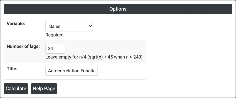
Figure 1 — Autocorrelation of monthly Sales for 24 lags (two years).
Output Descriptions
- Autocorrelation Function (graph) — a bar for each lag with the dashed significance limits.
- Autocorrelation Function: <variable> (table) — Lag, ACF, T and LBQ for each lag.
- PDF export via Download.
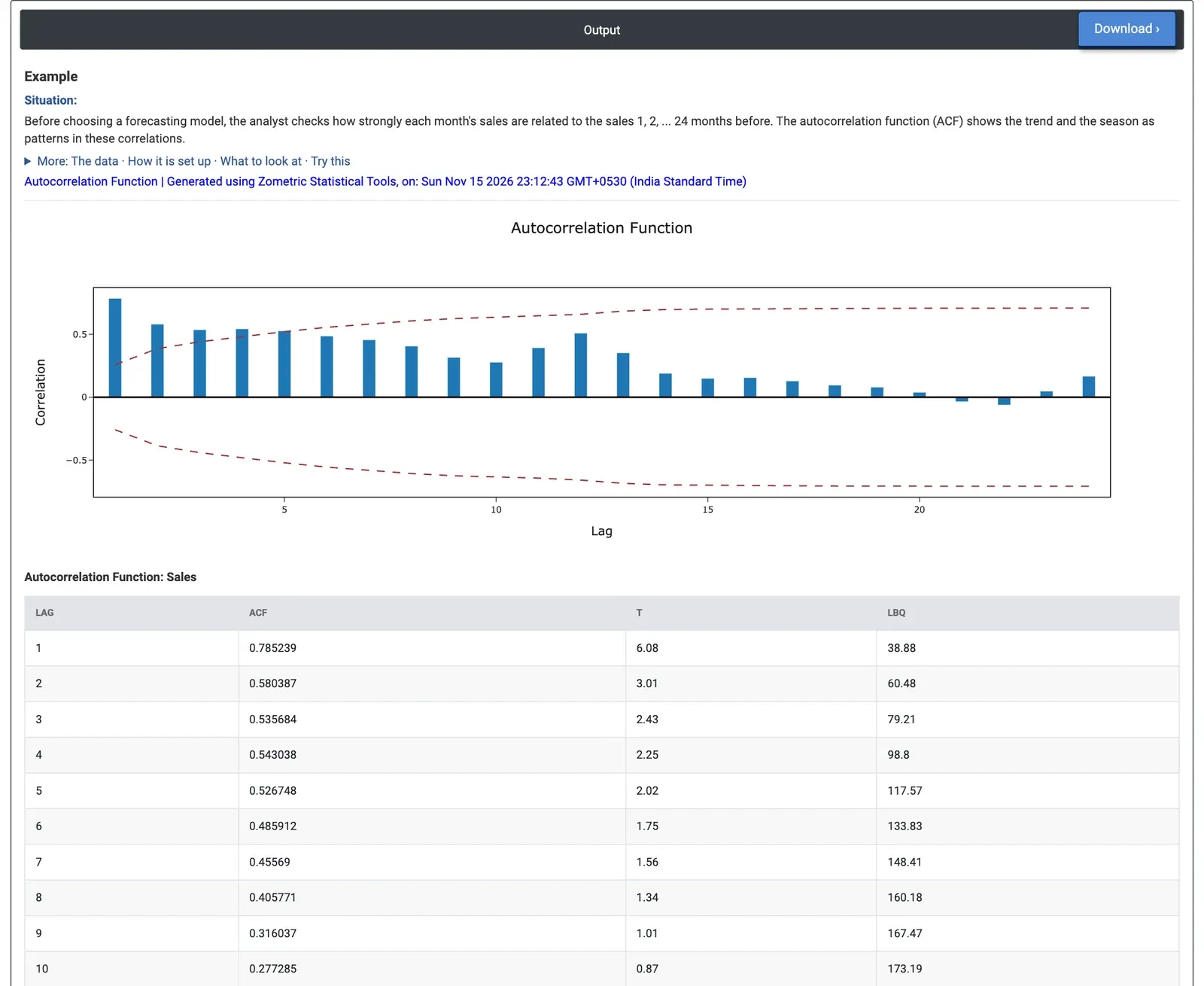
Figure 2 — ACF of monthly sales: a large lag 1 correlation of 0.79 that decays slowly, and a second rise at lag 12.
Worked Example
A consumer electronics distributor records unit sales every month, January 2020 to December 2024 (60 months). Before building a forecast, the sales analyst checks how each month relates to the 24 months before it. The analyst selects Variable = Sales and Number of lags = 24.
The lag 1 autocorrelation is 0.79 (T 6.08): neighbouring months are very alike. The correlations fall only slowly, from 0.58 at lag 2 to 0.49 at lag 6, and lags 1 to 5 are outside the significance limits. This slow decay is the mark of a trend: sales are not stationary. After a low of 0.28 at lag 10 the ACF rises again to 0.51 at lag 12, the yearly season; that bar stays inside the limits, which are wide by then (±0.66) because of the large earlier correlations. LBQ reaches 228.1 at lag 24, far above 36.4, the 5% chi-square critical value with 24 degrees of freedom, so there is a strong time pattern to model.
For the forecast, this means the series should be differenced (here seasonally, by 12 months) or the trend modelled directly. On the 12-month differences of Sales the slow decay is gone: the ACF is 0.47 at lag 1 and no other lag up to 11 is outside the limits, which is why the ARIMA example uses an AR(1) term on the seasonally differenced series. The ACF of Advertising Spend has an even stronger yearly peak: 0.59 at lag 12 (T 2.52).