
Binary Fitted Line Plot
On this page
Purpose
Binary Fitted Line Plot models how the probability of a yes/no outcome changes with one continuous predictor, and draws the fitted S-shaped curve over the data. Use it when the result is pass/fail, defective/good or caked/not caked, and you want to know how far a setting such as temperature, humidity or dose must move before the event becomes likely.
Key Capabilities
- Accepts raw data (one row per unit with a yes/no column) or summarised data (number of events and number of trials per row).
- Logit, probit or complementary log-log link.
- Regression equation, deviance ANOVA table, model summary, coefficients with confidence intervals and, for the logit link, the odds ratio for any increment of the predictor.
- Plot of the fitted probability curve with optional observed proportions and confidence band.
- Table of unusual observations (large residuals or unusual predictor values) and optional residual plots.
- Optional frequency column for data with repeated rows.
Statistical Methods
The tool fits a binary logistic regression with one predictor as a generalised linear model with a binomial distribution, by maximum likelihood (iteratively reweighted least squares). With the logit link, P(event) = exp(b₀ + b₁x) / (1 + exp(b₀ + b₁x)); with probit, P = Φ(b₀ + b₁x); with complementary log-log, P = 1 − exp(−exp(b₀ + b₁x)). In raw-data format, rows whose response equals the Event value count as events and all others as non-events.
The ANOVA table tests the predictor by the drop in deviance: χ² = null deviance − residual deviance, with 1 degree of freedom. Deviance R-Sq is the share of the null deviance explained. The coefficient table gives Wald z-values and confidence intervals b ± z·SE; the odds ratio for an increment Δ is exp(b₁·Δ), with interval exp(Δ × the limits of b₁). Area Under ROC Curve is the chance that a randomly chosen event has a higher fitted probability than a randomly chosen non-event (0.5 = no discrimination, 1 = perfect).
The confidence band around the curve uses the standard error of the linear predictor, transformed back to the probability scale. In the unusual observations table, a standardised residual beyond ±2 is flagged R and a leverage above 3p/n is flagged X. With raw data the observed proportions on the plot are the event rates within up to 10 groups of equal size along the predictor.
Input Fields & Options
Field | Description |
Data format | Binary response (one row per observation, default) or Event/Trial (one row per setting with a count of events and a count of trials). |
Response / Event value | Binary response format: the column holding the outcome, and the value in it that counts as the event (e.g. Yes, Fail, 1). |
Number of events / Number of trials | Event/Trial format: the columns with the count of events and the number of units tested on each row. |
Event name | Optional label for the event, used in the equation and plot axis, e.g. Caked. Blank: the Event value (Binary response format) or the name of the events column (Event/Trial format). |
Predictor (continuous) | Numeric predictor. Required. |
Link function | Logit (default), Probit or Complementary log-log. |
Confidence level | Default 95. |
Type of confidence interval | Two-sided (default), Lower bound or Upper bound; applies to coefficients, odds ratios and the curve band. |
Frequency (optional) | Column with the number of times each row occurs. |
Increment for odds ratio | Change in the predictor for which the odds ratio is reported. Default 1. Logit link only. |
Display observed proportions / Display confidence interval | Add the observed event proportions and the confidence band to the plot. Off by default. |
Residuals for plots | Regular or Deviance residuals for the residual plots. |
Histogram of residuals / Normal probability plot of residuals / Residuals versus order / Three in one | Residual plots; Three in one draws all three together. |
Residuals versus the variables | Plot the residuals against a chosen column. |
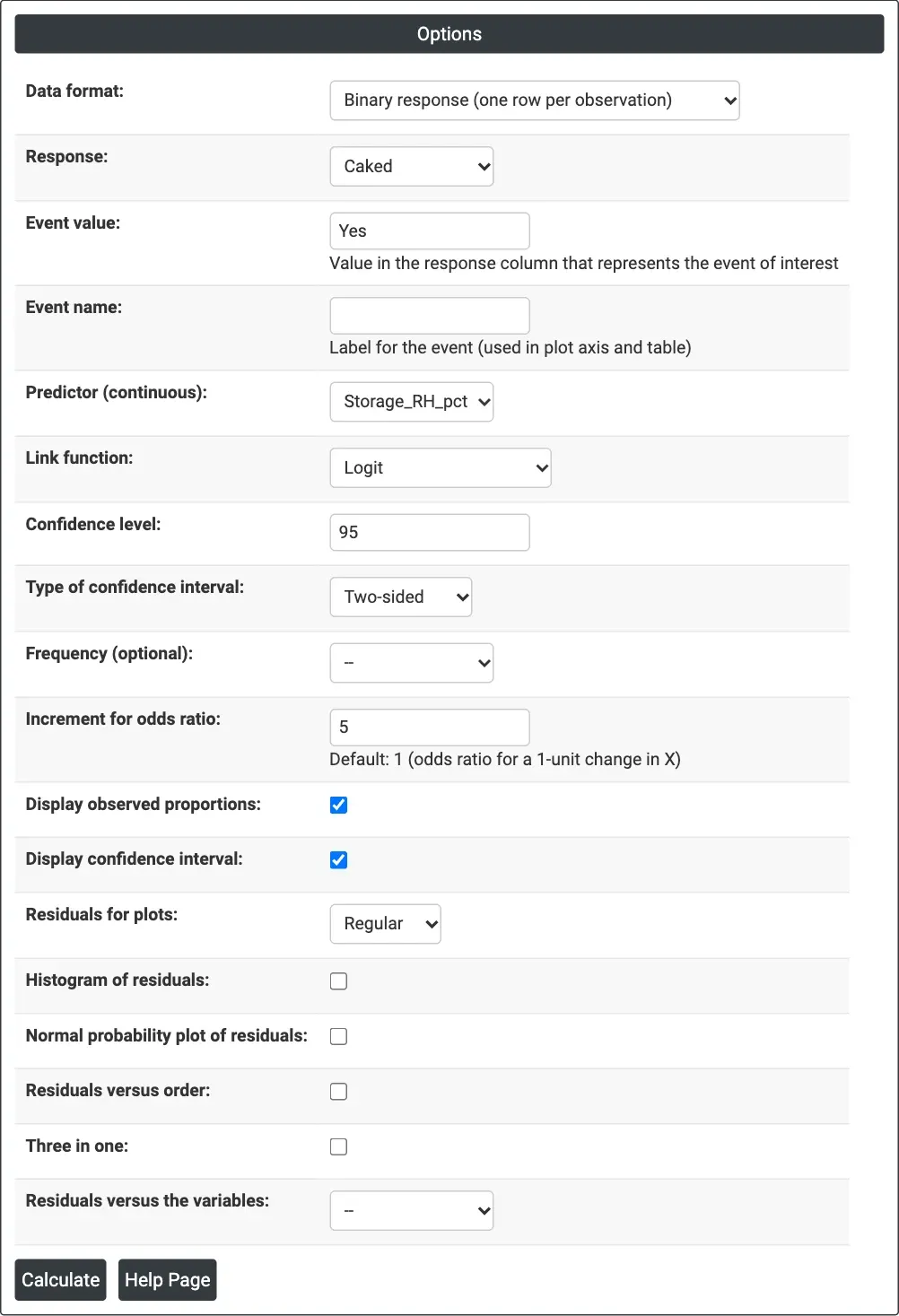
Figure 1 — Options for the bag caking example: Caked as the response with event Yes, Storage_RH_pct as the predictor, logit link, odds ratio for a 5-point increase in humidity.
Output Descriptions
- Regression Equation — the fitted probability of the event as a function of the predictor.
- Analysis of Variance — deviance test of the predictor (Adj Dev, Chi-Square, P-Value), with error and total deviance.
- Model Summary — Deviance R-Sq, Deviance R-Sq(adj), AIC, AICc, BIC and Area Under ROC Curve.
- Coefficients — Coef, SE Coef, Z-Value, P-Value and confidence limits for the constant and the predictor.
- Odds Ratios for Continuous Predictors (or Odds Ratios (Increment=Δ)) — logit link only.
- Binary Fitted Line Plot — fitted probability curve, with observed proportions and the confidence band if ticked.
- Fits and Diagnostics for Unusual Observations — rows flagged R (large residual) or X (unusual X).
- Residual plots, if selected.
- PDF export via Download.
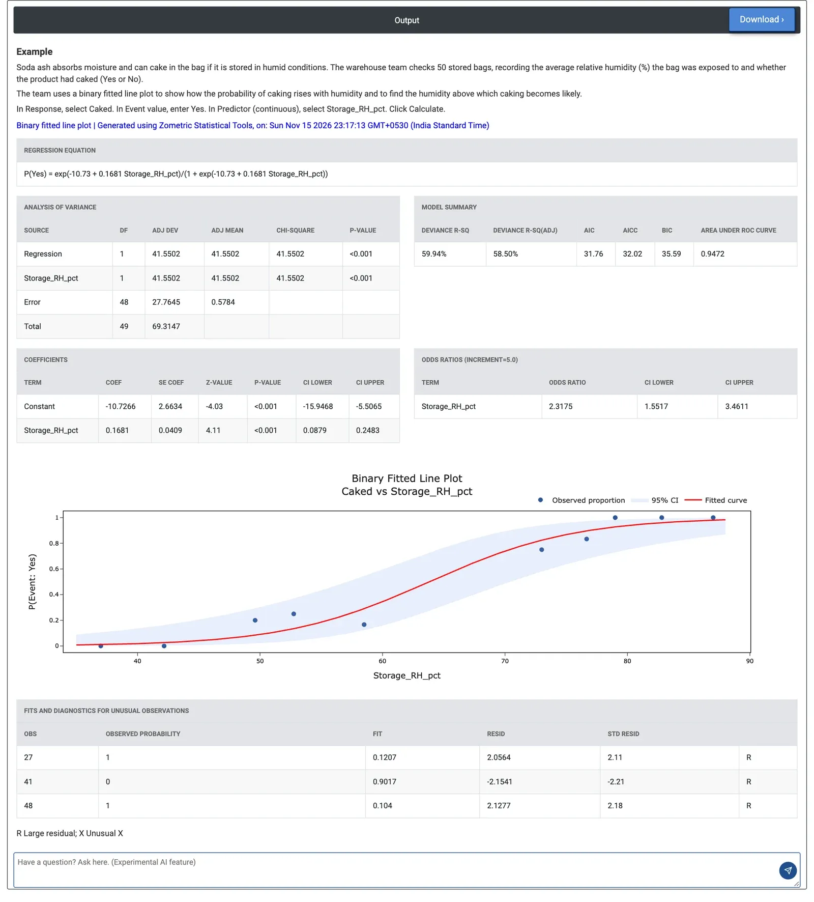
Figure 2 — Binary fitted line plot of the chance of caking against storage humidity: the curve passes 50% at about 64% RH.
Worked Example
Soda ash can cake in the bag when stored in humid conditions. A warehouse team checks 50 stored bags, noting the average relative humidity each bag was exposed to (Storage_RH_pct, 35 to 88%) and whether the product had caked (Caked: 25 Yes, 25 No). They select Caked as the response with Event value Yes, Storage_RH_pct as the predictor, keep the logit link, set the odds ratio increment to 5 and tick both display options.
Humidity has a clear effect: the deviance chi-square is 41.55 with p < 0.001, Deviance R-Sq is 59.94% and the area under the ROC curve is 0.9472, so humidity separates caked from sound bags well. The equation is P(Yes) = exp(−10.73 + 0.1681 RH) / (1 + exp(−10.73 + 0.1681 RH)). Each 5-point rise in humidity multiplies the odds of caking by 2.32 (95% CI 1.55 to 3.46). From the equation, the chance of caking is about 19% at 55% RH, 50% at 63.8% RH and 74% at 70% RH.
Three bags are flagged as unusual: two caked at low fitted probabilities (0.12 and 0.10) and one stayed sound at 0.90; worth checking for other causes such as damaged liners. To keep the caking risk below about 10%, the curve points to storage below roughly 51% RH. Switching to the probit link gives almost the same fit (Deviance R-Sq 60.50%).