
Binned Scatterplot
On this page
Purpose
A Binned Scatterplot divides the X–Y plane into a grid of rectangles (bins), counts the points in each one and colours the rectangle by the count. It shows where most of the data fall and how two variables move together, even when a normal scatterplot is a blur of overlapping points. Use it for large data sets from inline measurement or test benches, or to see at a glance which combinations of two properties are common and which are rare.
Key Capabilities
- Two-dimensional histogram of any two numeric columns.
- Number of bins on each axis set by you or chosen automatically.
- Colour bar showing the count for each colour, with a choice of colour scales.
- Data Options to exclude rows, or keep only rows, by row number or by a condition.
- Interactive graph: hover over a cell to see its X range, Y range and count; zoom and download as an image.
Statistical Methods
Both columns are converted to numbers and rows where either value is missing or non-numeric are dropped; at least two complete rows are needed. The graph is a two-dimensional histogram drawn by Plotly: each point is counted in the rectangle that contains it, and the colour of the rectangle shows the count. X axis bins and Y axis bins give the largest number of bins wanted on each axis; the graph then rounds the bin width to a tidy value (for example 20, 50 or 200), so the number of bins shown can be smaller than the number entered. Left blank, the bin sizes are chosen automatically from the data.
Reading the graph: a band of filled cells running from bottom left to top right means the two variables rise together; from top left to bottom right, one falls as the other rises. The brightest cells show the most common combination. Isolated cells far from the band are unusual points worth checking. The picture depends on the bin sizes: too few bins hide structure, too many leave most cells with 0 or 1 point. Counts are not a test of correlation; use Correlation or Regression to put a number on the relationship.
Input Fields & Options
Field | Description |
X-axis column | Required. Numeric column for the horizontal axis. |
Y-axis column | Required. Numeric column for the vertical axis. |
X axis bins / Y axis bins | Optional, 2 to 200. The largest number of bins on that axis; auto-calculated if left blank. |
Title | Title shown on the graph. Default Binned Scatterplot. |
Color scale | Colour scale for the counts. Default Viridis (dark for low counts, yellow for high). |
Data Options: Subset (optional) | Exclude matching rows (default) or Include only matching rows, matched by Row numbers (e.g. 3,7,12-15, using the original grid row numbers) and/or a Condition (e.g. Batch_Type == "Standard"). Has no effect unless Row numbers or Condition is filled in. |
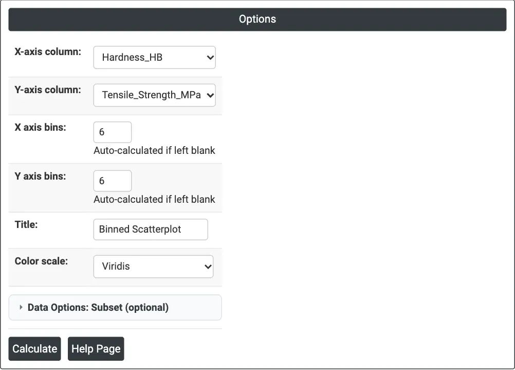
Figure 1 — Hardness on the X axis and tensile strength on the Y axis, with up to 6 bins on each axis.
Output Descriptions
- Binned Scatterplot — a grid of coloured rectangles over the X and Y ranges, with a Count colour bar.
- PDF export via Download.
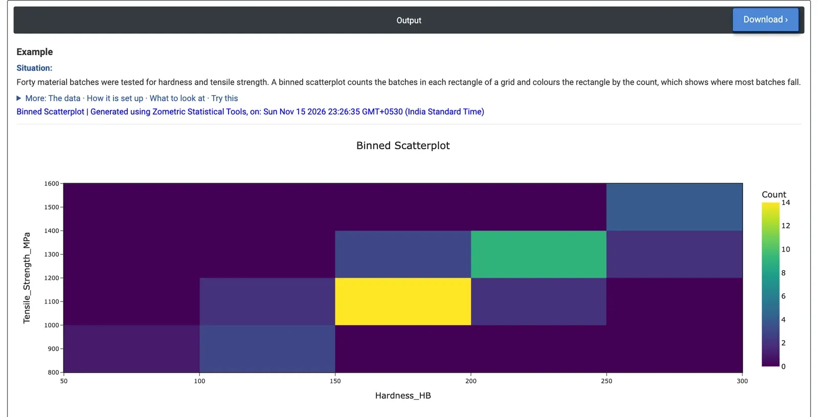
Figure 2 — Counts of 40 material batches by hardness and tensile strength: the busiest cell holds 14 batches.
Worked Example
A materials lab has tested 40 material batches for Brinell hardness and tensile strength. The metallurgist wants to see where most batches fall and whether hardness can stand in for the slower tensile test. The metallurgist selects X-axis column = Hardness_HB and Y-axis column = Tensile_Strength_MPa, and enters 6 for both X axis bins and Y axis bins. The graph rounds these to bins 50 HB wide (50 to 300 HB) and 200 MPa high (800 to 1,600 MPa).
The filled cells form a band from bottom left to top right: harder batches are stronger (the correlation of the two columns is 0.99). The busiest cell, 150 to 200 HB with 1,000 to 1,200 MPa, holds 14 of the 40 batches. Next come 200 to 250 HB with 1,200 to 1,400 MPa (9 batches) and 250 to 300 HB with 1,400 to 1,600 MPa (4 batches). One batch sits alone at 50 to 100 HB and below 1,000 MPa: the softest batch, at 80.1 HB and 822.6 MPa, a batch worth checking.
For the decision this means hardness tracks strength closely across the whole range, so it can serve as a quick screening test, with tensile tests kept for confirmation. With 12 bins on each axis the graph uses bins of 20 HB and 100 MPa; the band breaks into smaller cells and the largest count drops to 7, which shows the spread within the band in more detail.