
Chi-Square Test of Independence (Cross Tabulation)
On this page
Purpose
The Chi-Square Test of Independence checks whether two categorical variables are related, for example whether the mix of defect types depends on the shift, the supplier or the line. Enter a table of counts you have already summarised, or the raw records with one row per unit, and the tool tests the association and shows which cells drive it.
Key Capabilities
- Summarised two-way table (one column per column category, one row per row category) or raw categorical data with optional frequencies.
- Pearson and likelihood-ratio chi-square tests.
- Optional tables of expected counts, contributions to chi-square, raw, standardised and adjusted residuals, and row, column and total percents.
- Optional guided interpretation: summary report with percentage profiles and % difference charts, diagnostic report and report card.
- Data Options: subset the rows before the analysis.
Statistical Methods
For an r × c table of observed counts O with row totals Rᵢ, column totals Cⱼ and grand total N, the expected count under independence is Eᵢⱼ = Rᵢ·Cⱼ / N. The Pearson statistic is χ² = Σ (O − E)² / E, and the likelihood-ratio statistic is G² = 2 Σ O·ln(O / E). Both are compared with a chi-square distribution with (r − 1)(c − 1) degrees of freedom. A small p-value means the row and column variables are associated: the column mix is not the same in every row.
Each cell's contribution (O − E)² / E shows where the association comes from. The raw residual is O − E, the standardised residual (O − E) / √E, and the adjusted residual (O − E) / √(E(1 − Rᵢ/N)(1 − Cⱼ/N)), which is roughly standard normal: values beyond about ±2 mark cells that differ clearly from independence. With raw data the tool first cross-tabulates the two columns, summing the frequency column if one is given; blank cells are left out. A row or column with a total of zero must be removed. The p-value is reliable when the expected counts are not too small; the guided interpretation checks this.
Input Fields & Options
Field | Description |
Data | Summarized data in a two-way table (default) or Raw data (categorical variables). |
Columns (one per column-category) | Table layout: two or more numeric columns, each holding the counts for one category of the column variable, one row per row category. Required. |
Row labels | Table layout, optional: a column naming each row category; blank gives Row 1, Row 2, … |
Rows / Columns / Frequencies (optional) | Raw layout: the two categorical columns, and an optional column of counts for each record. |
Statistics | Expected cell counts and Each cell's contribution to chi-square (ticked by default); Raw residuals, Standardized residuals, Adjusted residuals, Row percents, Column percents, Total percents. |
Data Options: Subset (optional) | Exclude matching rows (default) or Include only matching rows, by row numbers and/or a condition. |
Show guided interpretation | Adds a plain-language Summary, Diagnostic and Report Card; Difference between the % defectives with practical value is an optional input for it. |
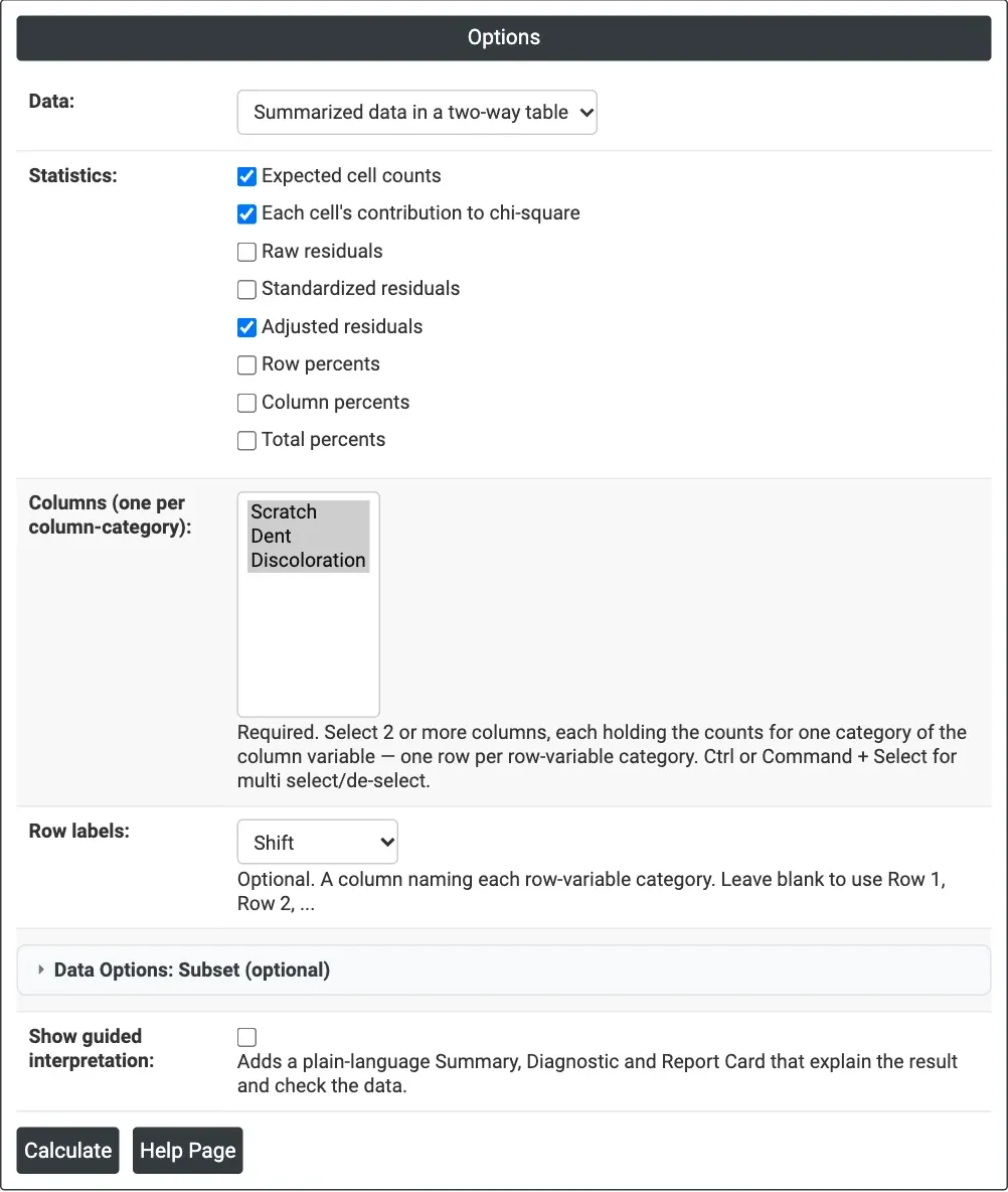
Figure 1 — Options for the defect-type example: a summarised table with the Scratch, Dent and Discoloration counts as columns and Shift as row labels, adjusted residuals ticked.
Output Descriptions
- Observed Counts — the table with row and column totals (All).
- Expected Counts and Contribution to Chi-Square — when ticked.
- Chi-Square Tests — Chi-Sq, DF and P-Value of the Pearson and likelihood-ratio tests.
- Raw Residuals, Standardized Residuals, Adjusted Residuals, Row Percents, Column Percents and Total Percents — when ticked.
- Summary Report, Diagnostic Report and Report Card — with guided interpretation.
- PDF export via Download.
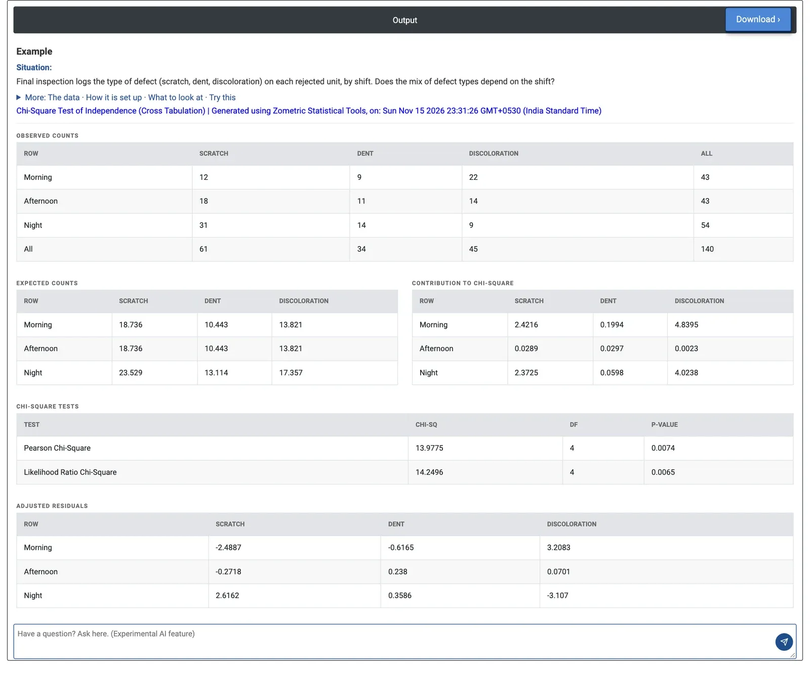
Figure 2 — Defect type by shift: Pearson chi-square 13.98 with 4 DF, p = 0.0074; the adjusted residuals point to discoloration on the morning shift and scratches on the night shift.
Worked Example
Final inspection records the type of defect on each rejected unit, by shift: 140 rejects in all. The quality team wants to know whether the mix of defect types depends on the shift. They enter the counts as a table with one column per defect type (Scratch, Dent, Discoloration) and Shift as row labels, and tick Adjusted residuals as well as the default statistics.
The defect mix does depend on the shift: Pearson chi-square 13.98 on 4 DF, p = 0.0074 (likelihood ratio 14.25, p = 0.0065). The contributions show where: discoloration on the morning shift (4.84; 22 observed against 13.8 expected) and on the night shift (4.02; 9 against 17.4), then scratches on the morning (2.42; 12 against 18.7) and night shifts (2.37; 31 against 23.5). The afternoon shift matches the overall mix, and dents are spread evenly.
The adjusted residuals confirm it: 3.21 for morning discoloration and 2.62 for night scratches are well beyond 2. The team looks at what changes at the start of the day (for example warm-up or a different paint batch) for discoloration, and at handling and lighting on the night shift for scratches. All expected counts are above 10, so the p-value can be trusted.