
Cluster K-Means
On this page
Purpose
Cluster K-Means splits observations into a fixed number of groups (K) so that the observations in each group are as alike as possible on the variables you choose. Use it when you expect a known number of groups, for example to sort material batches, parts or suppliers into types from several measured properties, or to check whether a label you already use (grade, line, shift) shows up in the measurements at all.
Key Capabilities
- Groups observations on two or more numeric variables into K clusters that you set.
- Optional standardisation, so that a variable measured in large units does not dominate the grouping.
- Several random starting points; the best solution (smallest within-cluster spread) is kept, and the same data always give the same result.
- Reports the final partition (size, within-cluster sum of squares, average and maximum distance from the centroid), the centroid of every cluster in the original units, the cluster of every observation, and the percentage of the total variation explained by the clusters.
- Scatter plot of the first two selected variables, coloured by cluster.
Statistical Methods
Rows with a missing or non-numeric value in any selected variable are dropped. When Standardize variables is ticked, each variable is converted to z = (x − mean) / s, using the sample standard deviation s, so that every variable has mean 0 and standard deviation 1 before clustering.
The K-means algorithm (Lloyd's method) assigns each observation to the nearest cluster centre by Euclidean distance, recomputes each centre as the mean of its members, and repeats until the assignments stop changing. Starting centres are chosen with the k-means++ rule. Because the result can depend on the start, the algorithm is run as many times as Number of random starts and the run with the smallest within-cluster sum of squares is kept. A fixed random seed is used, so results repeat exactly.
The percentage of variation explained by the clusters is (total SS − within-cluster SS) / total SS × 100, where total SS is the sum of squared distances of all observations from the overall mean and within-cluster SS is the sum of squared distances from each observation to its own cluster centre. Both are measured on the data as clustered (standardised when that option is ticked). A higher figure means more distinct, tighter groups, but it always rises as K grows, so compare it across K with care. Centroids are converted back to the original units for reporting. The final partition gives, for each cluster, the number of observations, the within-cluster sum of squares, and the average and maximum distance of its members from the centroid; these distances, and the distance of each observation in the membership table, are Euclidean distances in the units clustered (standardised when that option is ticked), as in Minitab.
Input Fields & Options
Field | Description |
Variables | Two or more numeric columns to cluster on. Ctrl or Command + click to select several. |
Number of clusters (K) | How many groups to form. Default 3; minimum 2. You need at least K complete observations. |
Standardize variables | Ticked by default. Puts every variable on the same scale (mean 0, standard deviation 1) before clustering. Untick only when all variables share the same units and you want larger-spread variables to carry more weight. |
Number of random starts | How many starting points to try; the best result is kept. Default 10, 1 to 100. |
Title | Title shown on the plot and output. Default Cluster K-Means. |
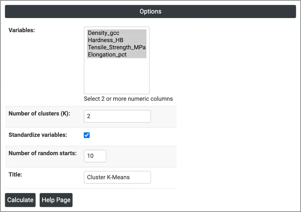
Figure 1 — Options for the example: the four property columns, K = 2, standardised, 10 random starts.
Output Descriptions
- Cluster K-Means plot — scatter plot of the first selected variable (x) against the second (y), each point coloured by its cluster.
- % variation explained by clusters — the share of total variation that lies between the clusters rather than within them.
- Final Partition — for each cluster: Number of observations, Within cluster sum of squares, Average distance from centroid and Maximum distance from centroid.
- Cluster Centroids — for each cluster, its number N of observations and the mean of each variable in the original units.
- Cluster Membership — each observation (by worksheet row), its cluster and its distance from that cluster's centroid.
- PDF export via Download.
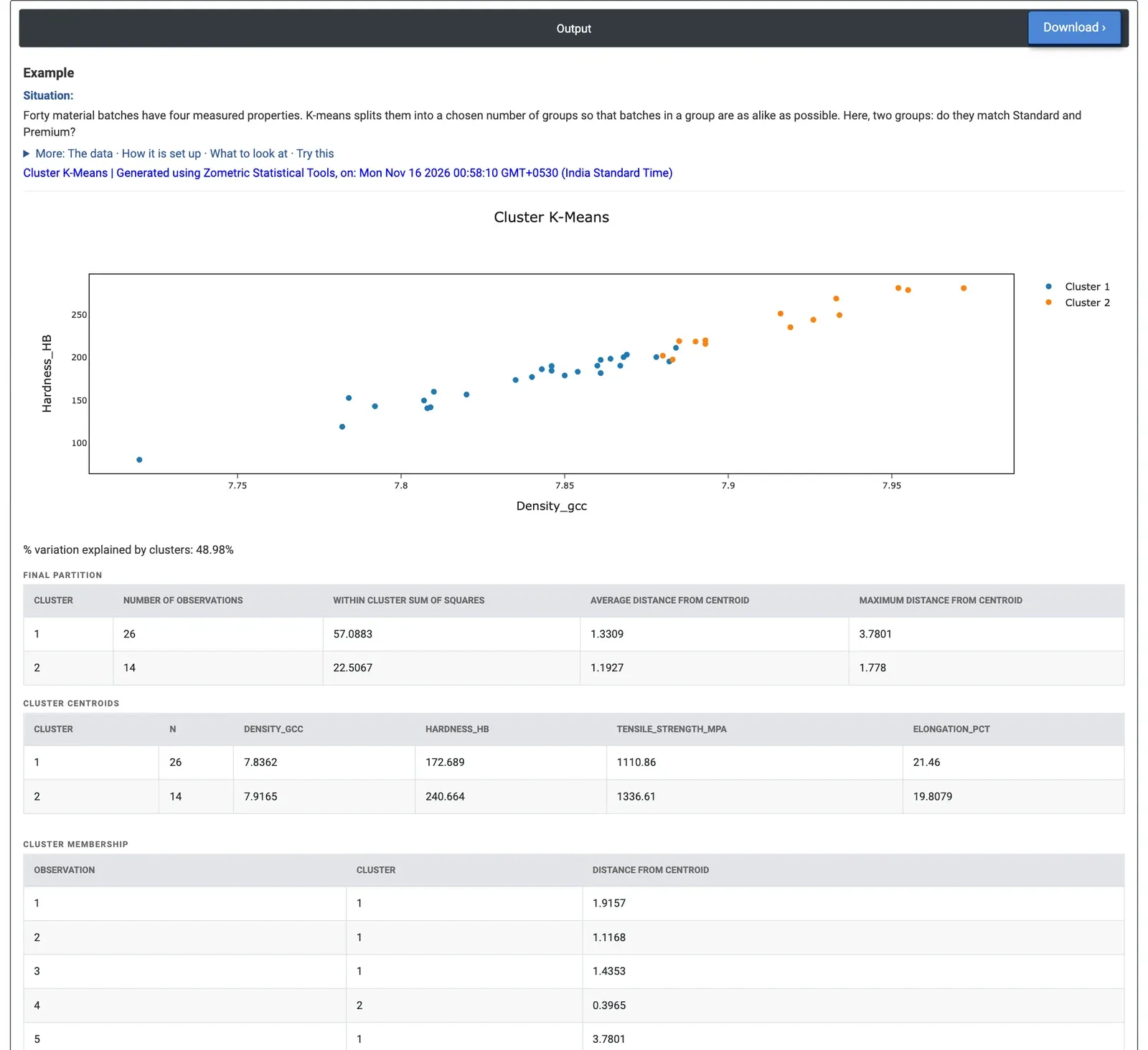
Figure 2 — Two clusters of 40 material batches: Cluster 2 (14 batches) is harder and stronger; the clusters explain 48.98% of the variation. The final partition, centroids and the start of the membership table follow the plot.
Worked Example
A materials lab has 40 batches, each measured for density (g/cc), hardness (HB), tensile strength (MPa) and elongation (%). The batches are sold as Standard or Premium, 20 of each. The lab wants to know whether the measurements alone fall into two natural groups, and whether those groups match the batch type. They select the four property columns, set Number of clusters (K) = 2, keep Standardize variables ticked (tensile strength, in the hundreds, would otherwise dominate) and keep 10 random starts.
The clusters explain 48.98% of the variation. Cluster 2 holds 14 batches that are harder and stronger (mean 240.7 HB and 1,336.6 MPa) and slightly less ductile (19.8% elongation); Cluster 1 holds 26 batches with means of 172.7 HB, 1,110.9 MPa and 21.5% elongation. The density centroids differ only a little (7.92 against 7.84 g/cc). In the final partition Cluster 2 is the tighter group (average distance from centroid 1.19 against 1.33 standardised units); the most distant member of Cluster 1, row 5, is 3.78 units from its centroid, an unusual batch worth checking. Comparing with the batch type column, Cluster 2 contains 11 Premium and 3 Standard batches, and Cluster 1 contains 17 Standard and 9 Premium, so 28 of 40 batches fall in the cluster that matches their type.
For the lab this means the strongest batches form a clear group, but many Premium batches are no harder or stronger than Standard ones: the label is not fully supported by the properties. With K = 3 the variation explained rises to 69.66% and a soft, weak group of 9 batches (138.2 HB, 995.9 MPa) separates from a middle group of 23 and a top group of 8. Unticking Standardize variables changes the split to 19 and 21 batches, because tensile strength then carries most of the weight. To build a rule that uses the known types, run Discriminant Analysis on the same data.