
Cluster Observations
On this page
Purpose
Cluster Observations groups observations (rows) that are alike across several numeric variables, without needing to know the number of groups in advance. It joins the most similar observations step by step and draws the result as a dendrogram (tree), so you can see how many natural groups there are and which observations belong together. Use it to look for natural families of batches, parts, suppliers or production runs, or to spot an observation that does not fit any group.
Key Capabilities
- Hierarchical (agglomerative) clustering of observations on two or more numeric variables.
- Seven linkage methods: Single, Complete, Average, Centroid, Median, McQuitty and Ward.
- Five distance measures: Euclidean, Squared Euclidean, Manhattan (City Block), Cosine and Correlation.
- Optional standardisation so that variables in different units count equally.
- Dendrogram of the whole joining sequence, and an optional cluster assignment for each observation when you give a number of clusters.
Statistical Methods
Rows with a missing or non-numeric value in any selected variable are dropped; at least 3 observations are needed. When Standardize variables is ticked, each variable is converted to z = (x − mean) / s with the sample standard deviation s. The distance between every pair of observations is then computed with the chosen measure: Euclidean √Σ(xᵢ − yᵢ)², Squared Euclidean Σ(xᵢ − yᵢ)², Manhattan Σ|xᵢ − yᵢ|, Cosine 1 − cos(angle between the two rows) or Correlation 1 − r between the two rows.
Clustering starts with every observation as its own cluster and repeatedly merges the two closest clusters until one remains. The linkage method sets how the distance between two clusters is measured: Single uses the closest pair of members, Complete the farthest pair, Average the mean of all pairwise distances, McQuitty a weighted average, Centroid the distance between cluster centres, Median the distance between unweighted centres, and Ward merges the pair of clusters that gives the smallest increase in the within-cluster sum of squares. Ward, Centroid and Median need a Euclidean or Squared Euclidean distance; the tool refuses other combinations.
The height at which two branches join in the dendrogram is the distance between them at the time of merging, so long vertical branches mark well-separated groups. When Number of clusters is entered, the tree is cut at the level that gives that many clusters, and each observation is labelled with its cluster number.
Input Fields & Options
Field | Description |
Variables | Two or more numeric columns that describe each observation. Ctrl or Command + click to select several. |
Linkage method | How the distance between clusters is measured: Single, Complete, Average (default), Centroid, Median, McQuitty or Ward. |
Distance measure | How the distance between two observations is measured: Euclidean (default), Squared Euclidean, Manhattan (City Block), Cosine or Correlation. |
Standardize variables | Ticked by default. Scales every variable to mean 0 and standard deviation 1 first, so a variable in large units does not dominate. |
Number of clusters | Optional, 2 or more. Cuts the tree into this many clusters and adds the Cluster Assignments table. Leave empty to only show the dendrogram. |
Title | Title shown on the dendrogram. Default Cluster Observations. |
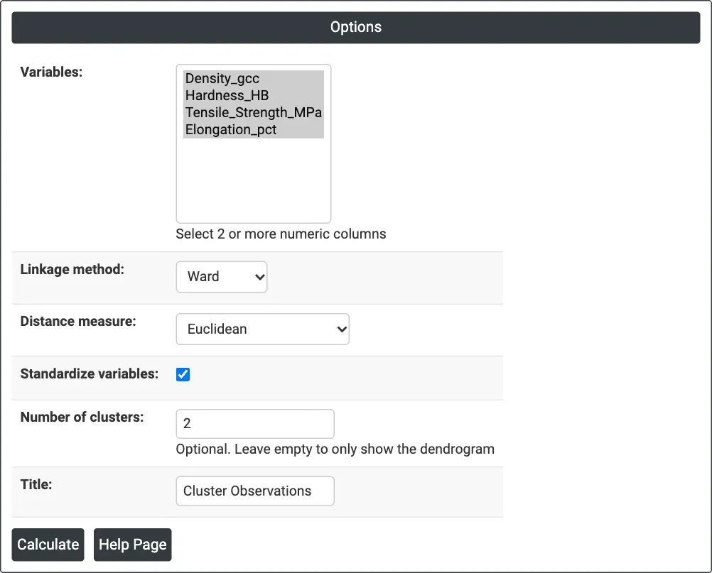
Figure 1 — Options for the example: four property columns, Ward linkage, Euclidean distance, standardised, 2 clusters.
Output Descriptions
- Dendrogram — the joining sequence. Observations (row numbers) are along the x-axis in tree order; the y-axis (Distance) shows the level at which branches join.
- Cluster Assignments — shown when Number of clusters is entered: each observation's row number and its cluster number.
- PDF export via Download.
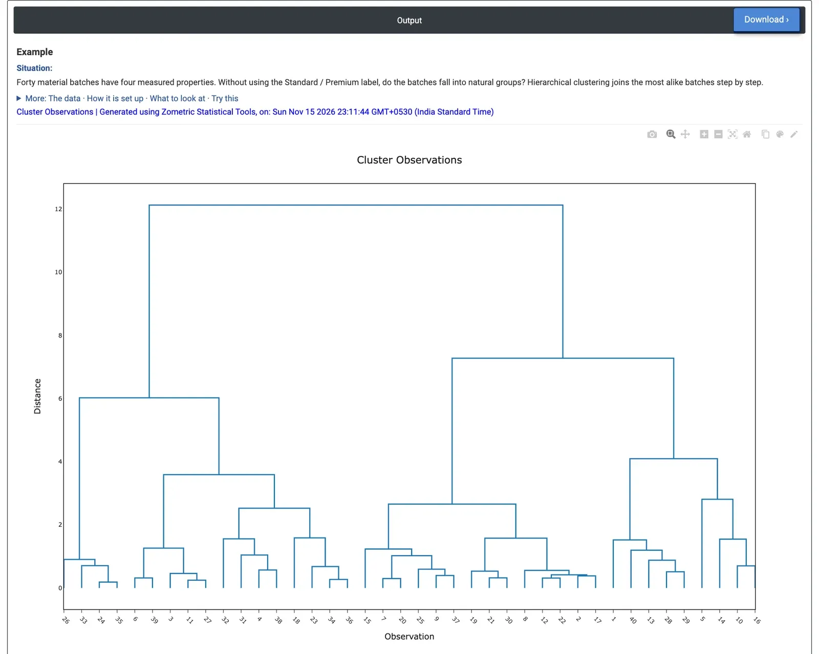
Figure 2 — Dendrogram of 40 material batches with Ward linkage: two main branches join at a distance of about 12.1.
Worked Example
A materials lab has 40 batches measured for density (g/cc), hardness (HB), tensile strength (MPa) and elongation (%). Without using the Standard or Premium label, the lab wants to know whether the batches fall into natural groups. They select the four property columns, choose Linkage method = Ward and Distance measure = Euclidean, keep Standardize variables ticked (density in g/cc and strength in MPa would otherwise not be comparable) and enter Number of clusters = 2.
The dendrogram shows two main branches that join at a distance of 12.1, well above the next joins (7.3 and 6.0), so two groups is a natural cut. Cluster 1 has 17 batches that are harder and stronger (mean 231.6 HB and 1,308 MPa, 19.8% elongation); Cluster 2 has 23 softer and more ductile batches (170.5 HB, 1,103 MPa, 21.7% elongation). Against the batch type, Cluster 1 holds 12 Premium and 5 Standard batches and Cluster 2 holds 15 Standard and 8 Premium: the clusters follow the type for only 27 of 40 batches.
For the lab, the properties overlap a lot between the two types, and a fair share of Standard batches are as strong as Premium ones. The choice of linkage matters: with Average linkage the two-cluster cut sets apart a single batch (row 5, 80.1 HB and 822.6 MPa, far softer than the rest) and puts the other 39 together, which is a useful way to find an outlier rather than groups. Cutting the Ward tree at 3 clusters separates a soft group of 9 batches (138.2 HB, 995.9 MPa).