
Attribute Acceptance Sampling (Compare)
On this page
Purpose
Attribute Acceptance Sampling (Compare) puts several single sampling plans for inspection by attributes side by side. Each plan is a sample size n and an acceptance number c: inspect n units at random from the lot and accept it if c or fewer are defective. You enter the plans you are considering, for example the plan in use today, a customer's plan and the plan from Attribute Acceptance Sampling (Create), with your AQL and RQL, and the tool shows how often each plan accepts good and bad lots, and with a lot size how much defective product gets through and how much inspection each plan costs. Use it to choose between plans or to check whether an existing plan protects you.
Key Capabilities
- Any number of plans in one run, entered as matching lists of sample sizes and acceptance numbers.
- Probability of acceptance at the AQL and at the RQL for every plan.
- Operating characteristic (OC) curves of all plans on one plot.
- With a lot size: average outgoing quality (AOQ) and average total inspection (ATI) curves for each plan, for rectifying inspection.
- Quality levels in defectives per million (ppm).
- PDF export via Download.
Statistical Methods
For each plan the probability of accepting a lot with fraction defective p is the binomial probability of finding c or fewer defectives in n units: Pa(p) = Σ (k = 0 to c) C(n, k)·pᵏ·(1 − p)ⁿ⁻ᵏ. The table gives Pa at the AQL and at the RQL (both entered in ppm and divided by 1,000,000). One minus Pa(AQL) is the producer's risk, the chance of rejecting a good lot; Pa(RQL) is the consumer's risk, the chance of accepting a bad lot. A plan with a steeper OC curve separates good and bad lots better and needs a larger sample.
With a lot size N, the AOQ and ATI curves assume rectifying inspection: rejected lots are inspected 100% and defective units are replaced. Then AOQ(p) = p·Pa(p)·(N − n) / N, the average fraction defective leaving inspection, and ATI(p) = n + (1 − Pa(p))·(N − n), the average number of units inspected per lot. The peak of a plan's AOQ curve is its average outgoing quality limit (AOQL). All curves are drawn for lot quality from 0 to three times the RQL. Each c must be less than its n, each n smaller than the lot size, and the RQL larger than the AQL. The binomial model assumes the lot is large compared with the sample.
Input Fields & Options
Field | Description |
Units for quality level | Defectives Per Million (the only choice). |
Acceptable Quality Level (AQL) | Required, in ppm, e.g. 10000 for 1% defective. The quality level at which lots should usually be accepted. |
Rejectable Quality Level (RQL / LTPD) | Required, in ppm, larger than the AQL. The quality level at which lots should usually be rejected. |
Sample sizes (n) | Required. Space or comma-separated, e.g. “50 80 120”, one per plan. |
Acceptance numbers (c) | Required. Same count as sample sizes, e.g. “1 2 3”; the first c goes with the first n, and so on. |
Lot size | Optional, at least 2. Needed for the AOQ and ATI curves. |
Operating characteristic (OC) curve / Average outgoing quality (AOQ) curve / Average total inspection (ATI) curve | All ticked by default. The AOQ and ATI curves are drawn only when a lot size is entered. |
Title | Default Compare Acceptance Sampling by Attributes. |
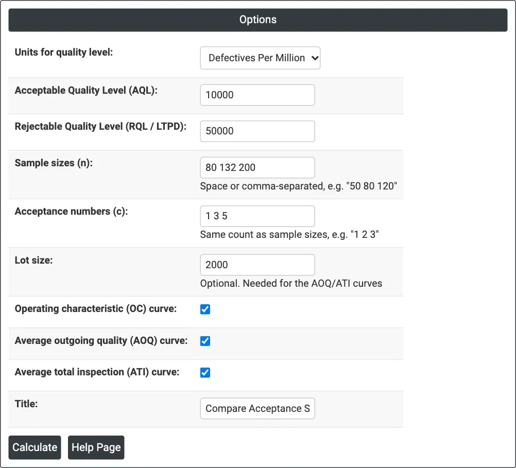
Figure 1 — Three plans (n = 80, 132, 200 with c = 1, 3, 5) compared at AQL 10,000 ppm and RQL 50,000 ppm for lots of 2,000.
Output Descriptions
- Plan table — Plan, n, c, P(accept | AQL) and P(accept | RQL) for each plan.
- Operating Characteristic (OC) Curves — probability of acceptance against lot defectives per million, one curve per plan.
- Average Outgoing Quality (AOQ) Curves — when a lot size is given: average outgoing proportion defective against lot defectives per million; each peak is that plan's AOQL.
- Average Total Inspection (ATI) Curves — when a lot size is given: average number of units inspected per lot.
- PDF export via Download.
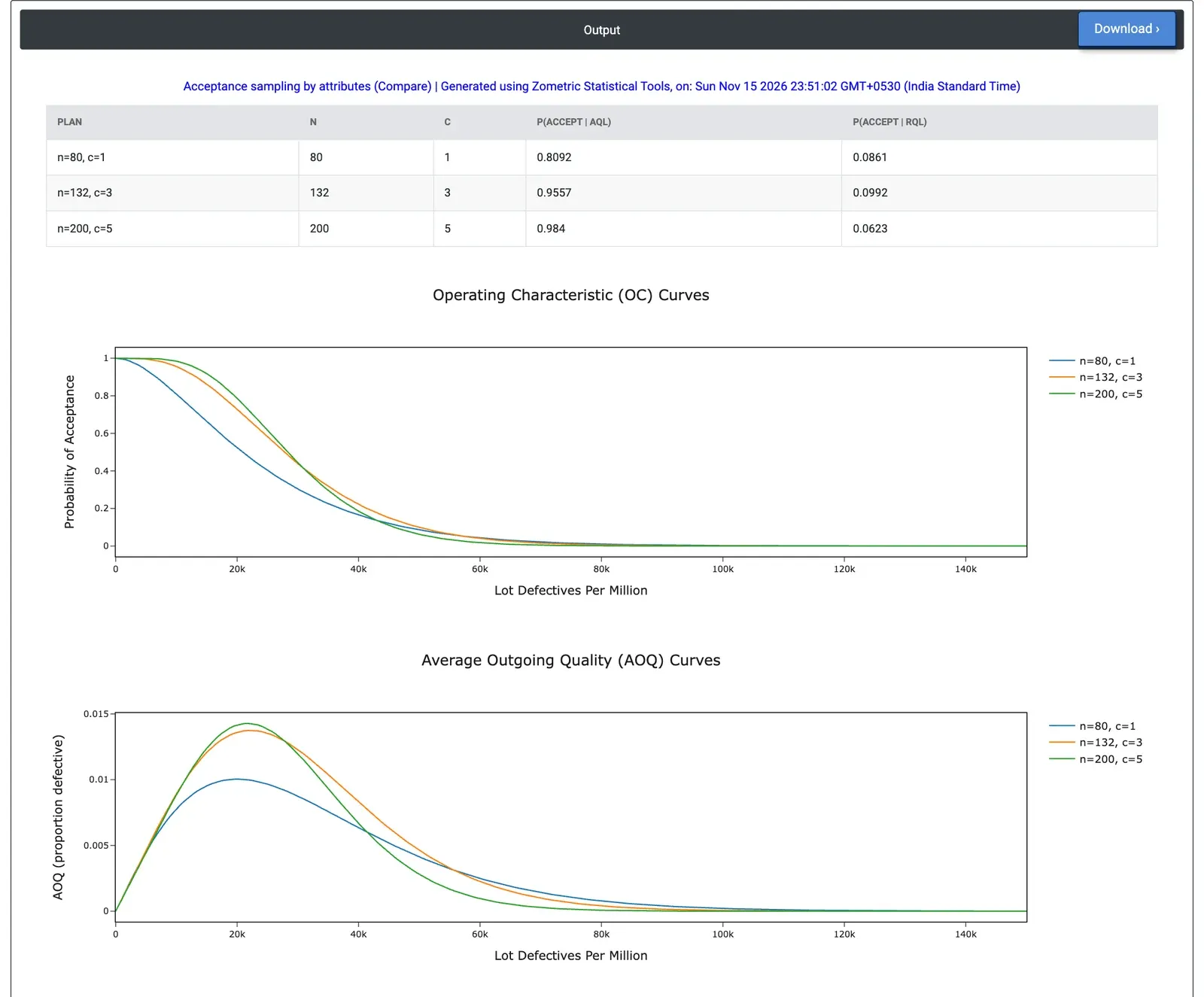
Figure 2 — The plan table, OC curves and AOQ curves for the three plans; n = 200, c = 5 has the steepest OC curve.
Worked Example
A supplier quality engineer receives moulded connectors in lots of 2,000 and checks them with a go/no-go gauge. Lots that are 1% defective (AQL 10,000 ppm) should pass and lots that are 5% defective (RQL 50,000 ppm) should be stopped. Three plans are on the table: the current plan n = 80, c = 1; the plan from Attribute Acceptance Sampling (Create), n = 132, c = 3; and a customer's plan, n = 200, c = 5. The engineer enters Sample sizes = 80 132 200, Acceptance numbers = 1 3 5 and Lot size = 2000.
The current plan accepts only 80.9% of lots at the AQL: about one good lot in five is rejected, which is unfair to the supplier and costly to sort. It accepts 8.6% of lots at the RQL. The plan n = 132, c = 3 accepts 95.6% at the AQL and 9.9% at the RQL, and n = 200, c = 5 accepts 98.4% and 6.2%, the best on both counts. On the OC plot its curve is the steepest.
The lot-size curves show the cost. When lots are at the AQL, the current plan inspects about 446 connectors per lot on average, because it sorts so many good lots, against about 215 for n = 132 and 229 for n = 200. The larger plans let a little more through at worst: their AOQ curves peak at about 0.0137 and 0.0143 (1.4% defective), against 0.0100 for the current plan, because they reject fewer lots for sorting. The engineer drops the current plan and picks n = 132, c = 3 or, if the customer insists, n = 200, c = 5 for about 14 more units per lot.