
Simple Correspondence Analysis
On this page
Purpose
Simple Correspondence Analysis turns a two-way table of counts into a map. Row categories and column categories are drawn as points, and categories that go together more often than chance would suggest sit close to each other. Use it to see the pattern in a large cross-table at a glance: which defect types go with which machines, which complaint categories go with which products, or which attributes customers link with which brands.
Key Capabilities
- Accepts raw data (one row per item with two categorical columns) or a contingency table already summarised as counts.
- Chi-square test of association between the row and column variables.
- Inertia table showing how much of the association each component (axis of the map) explains.
- Row and column contribution tables: quality, mass, inertia, coordinates, squared correlations and contributions for the number of components you choose.
- Five plots: symmetric plot of rows and columns, rows only, columns only, and asymmetric row or column plots.
Statistical Methods
With Categorical variables input, the tool cross-tabulates the row variable against the column variable, ignoring rows with a missing value. With Columns of a contingency table input, each selected column holds the counts for one column category and each row is a row category; rows or columns that total zero are dropped. Each variable needs at least 2 categories.
The counts are divided by the grand total n to give proportions P, with row masses r (row totals of P) and column masses c (column totals). The matrix of standardised residuals S = Dr^−½ (P − r cᵀ) Dc^−½ is split by singular value decomposition. Each singular value d gives one component with inertia d², and the number of components is the smaller of (rows − 1) and (columns − 1). Total inertia equals the chi-square statistic divided by n, and the tool reports chi-square = n × total inertia with (rows − 1)(columns − 1) degrees of freedom and its p-value. A small p-value means the rows and columns are associated, so the map shows a real pattern.
Principal coordinates for rows are Dr^−½ U D and for columns Dc^−½ V D. In the contribution tables, Mass is the category's share of the total count, Inert its share of the total inertia, Corr the squared cosine (how well one component shows the point), Qual the sum of Corr over the reported components, and Contr the share of a component's inertia that the point accounts for. Symmetric plots use principal coordinates for both sets of points; an asymmetric row plot shows rows in principal and columns in standard coordinates (principal divided by d), and an asymmetric column plot the reverse.
Input Fields & Options
Field | Description |
Input data | Categorical variables (default): one row per item. Columns of a contingency table: counts already summarised. The fields below change with this choice. |
Row variable / Column variable | For Categorical variables input: the two categorical columns to cross-tabulate. Both required and must be different. |
Contingency table columns | For contingency table input: two or more columns, each holding the counts for one column category, one row per row category. |
Row names | For contingency table input, optional: a column naming each row of the table. Blank uses Row 1, Row 2, and so on. |
Column names | For contingency table input, optional: a column listing one name per selected table column, in the same order. Blank uses the column headers. |
Number of components | How many components to report Coord, Corr and Contr for in the contribution tables. Default 2; 1 to 20, limited to the number of components available. |
Symmetric plot showing rows and columns | Ticked by default. Rows and columns on one map, both in principal coordinates. |
Symmetric plot showing rows only / columns only | Unticked by default. The same map with only one set of points. |
Asymmetric row plot / Asymmetric column plot | Unticked by default. Rows in principal and columns in standard coordinates, or the reverse. |
Title | Title shown on the plots. Default Simple Correspondence Analysis. |
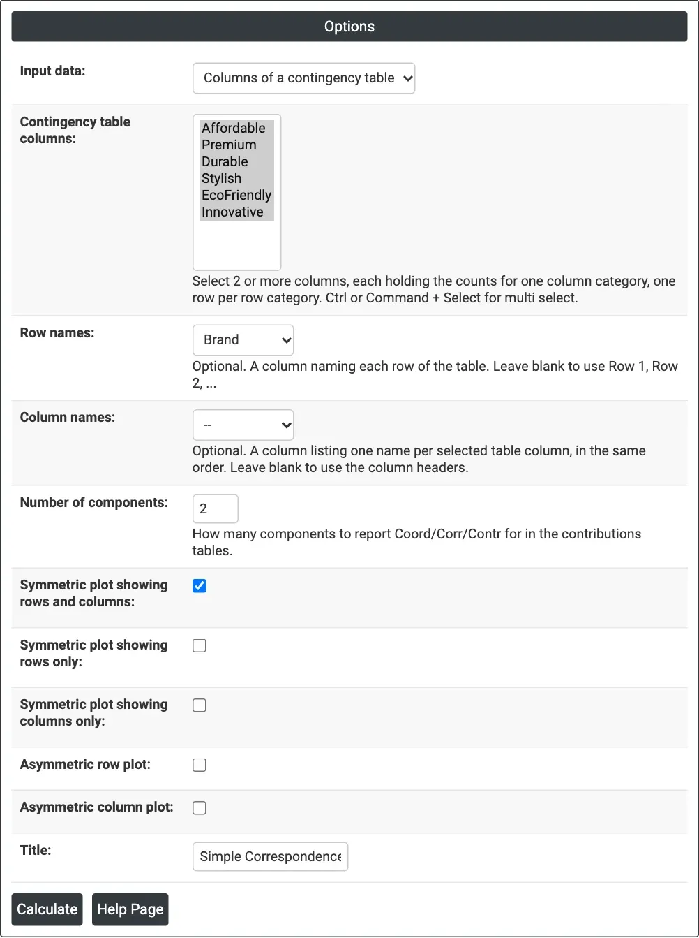
Figure 1 — Options for the brand-perception example: contingency table input with six attribute columns and Brand as the row names.
Output Descriptions
- Symmetric Plot, Row Plot, Column Plot, Asymmetric Row Plot, Asymmetric Column Plot — the plots ticked, with Component 1 and Component 2 as axes and the percentage of inertia each explains in the axis titles.
- Contingency Table — shown for contingency table input: the table as analysed.
- Chi-square, DF and P-value — the test of association between rows and columns.
- Analysis of Contingency Table — inertia, proportion and cumulative proportion for each axis, with a text histogram, and the total inertia.
- Row Contributions and Column Contributions — ID, Name, Qual, Mass, Inert, and Coord, Corr and Contr for each reported component.
- PDF export via Download.
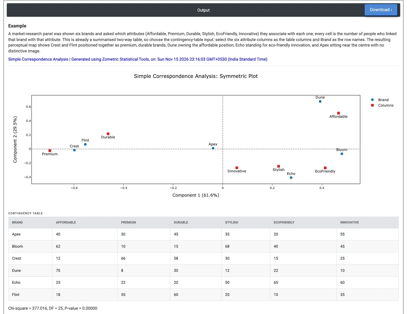
Figure 2 — Symmetric plot of six brands and six attributes: Crest and Flint sit with Premium and Durable, Dune with Affordable, Echo near EcoFriendly; chi-square 377.0 on 25 DF.
Worked Example
A market-research panel was shown six brands (Apex, Bloom, Crest, Dune, Echo and Flint) and asked which of six attributes they link with each one: Affordable, Premium, Durable, Stylish, EcoFriendly and Innovative. Each cell holds the number of people who linked that brand with that attribute. The marketing team wants to see each brand's position. Because the data are already a table of counts, they set Input data = Columns of a contingency table, select the six attribute columns as Contingency table columns and choose Brand as Row names, keeping the symmetric plot of rows and columns.
Chi-square is 377.016 with 25 degrees of freedom (p < 0.00001), so brand image clearly differs between brands. Component 1 carries 61.6% of the inertia and Component 2 29.5%, so the two-dimensional map shows 91.1% of the pattern. Component 1 runs from Premium (−0.698) and Durable (−0.462) on the left to Affordable (0.467) and EcoFriendly (0.414) on the right. Crest (−0.599) and Flint (−0.554) sit on the premium, durable side and are shown almost perfectly on this axis (Corr 0.94 and 0.98). Dune sits high on Component 2 (0.674), next to Affordable, and accounts for 62.2% of that component's inertia. Echo (0.276, −0.406) sits near EcoFriendly, Stylish and Innovative, and Bloom (0.481) leans towards Stylish and Affordable.
Apex sits near the centre (−0.039, 0.011) with a quality of only 0.038: its profile is close to the average of all brands, so it has no distinctive image. For the team, Crest and Flint compete for the same premium, durable position, Dune owns the affordable position, and Apex is the brand that needs a clearer message.