
Cox Regression (Fixed Covariates)
On this page
Purpose
Cox Regression (Fixed Covariates) relates the risk of failure to one or more measured factors, such as operating temperature, vibration, load or supplier, using life data in which some units have not yet failed. It reports a hazard ratio for each factor: how much the failure risk changes for each unit increase in that factor, with no need to choose a life distribution. Use it on field or test data to find which conditions shorten life and by how much.
Key Capabilities
- Proportional hazards model with one or more numeric covariates.
- Handles right-censored data: units still running when observation stopped.
- Coefficient, standard error, Z statistic and p-value for each covariate.
- Hazard ratio with a confidence interval at the level you choose.
- Survival plot for a unit at the average value of every covariate.
Statistical Methods
The model is the Cox proportional hazards model, h(t | Z) = h₀(t) · exp(β₁Z₁ + β₂Z₂ + ...), where h(t | Z) is the failure rate at time t for a unit with covariate values Z and h₀(t) is a baseline hazard that is not given any particular form. The coefficients β are estimated by maximising the partial likelihood (Breslow method for tied failure times), which uses only the order in which units fail and the units still at risk at each failure time. A censored unit counts as at risk up to its censoring time.
Standard errors come from the inverse of the Hessian of the log partial likelihood at the estimate. Each coefficient is tested with the Wald statistic Z = coef / SE against the standard normal distribution. The hazard ratio is exp(coef): the factor by which the failure rate is multiplied for a one-unit increase in that covariate, holding the others fixed. A hazard ratio above 1 means higher risk, below 1 lower risk. Its confidence interval is exp(coef ± z·SE), where z is the standard normal value for the confidence level. For a change of k units, the hazard ratio is exp(k · coef).
The model assumes that the effect of each covariate is the same at all times (proportional hazards) and that the effect on the log hazard is linear in the covariate. In the censoring column, rows equal to the censoring value are censored and every other row is a failure. The survival plot shows the fitted survival curve for a unit with every covariate at its sample mean; it starts at 1 at time 0 and steps down at each failure time.
Input Fields & Options
Field | Description |
Time variable | Required. Time to failure, or time to censoring for units still running. |
Use censoring column | Required. Rows equal to the censoring value are right-censored; every other row is a failure. Every row needs a value. |
Censoring value | The value in the censoring column that marks a unit still running when observation stopped. Default 0, so 1 = failure. |
Covariates (predictors) | One or more numeric predictor columns. Hold Ctrl or Command to select several. |
Confidence level (%) | For the hazard ratio confidence intervals. Default 95; 50 to 99.99. |
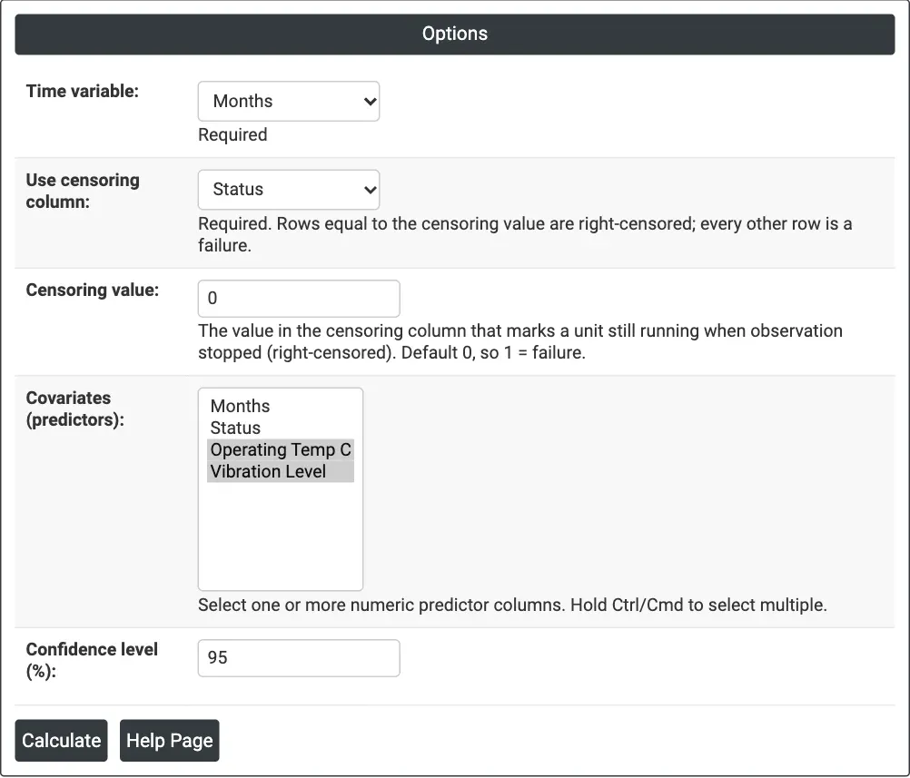
Figure 1 — Options for the example: Months as the time, Status as the censoring column (0 = still running), operating temperature and vibration as covariates.
Output Descriptions
- Model summary — Log-Likelihood, N (Observations) and N (Events), the number of failures.
- Coefficients — for each predictor: Coef, SE Coef, Z, P, Hazard Ratio and its lower and upper confidence limits.
- Cox Regression Survival Plot (at mean covariate values) — fitted survival probability against time for a unit at the average of each covariate.
- PDF export via Download.
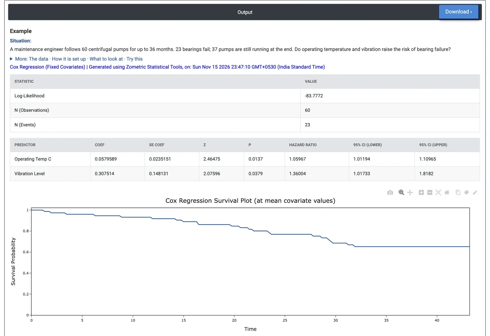
Figure 2 — Results for 60 pumps: hazard ratio 1.06 per °C of operating temperature and 1.36 per unit of vibration, both significant at the 5% level, and the survival curve for a pump at average temperature and vibration.
Worked Example
A maintenance engineer follows 60 centrifugal pumps for up to 36 months. 23 bearings fail; the other 37 pumps are still running at the end and are censored at 36 months. For each pump the engineer has the operating temperature (°C) and a measured vibration level. The engineer wants to know whether temperature and vibration raise the risk of bearing failure. The engineer sets Time variable = Months, Use censoring column = Status with Censoring value = 0, and selects Operating Temp C and Vibration Level as covariates at 95% confidence.
Operating temperature has a coefficient of 0.0580 (p = 0.0137) and a hazard ratio of 1.060 per °C (95% CI 1.012 to 1.110). Over 10 °C this is exp(10 × 0.0580) = 1.79: a pump running 10 °C hotter has about 1.8 times the failure risk. Vibration level has a coefficient of 0.3075 (p = 0.0379) and a hazard ratio of 1.360 per unit (95% CI 1.017 to 1.818): each extra unit of vibration raises the failure risk by about 36%. Both effects are significant at the 5% level, and neither confidence interval includes 1.
For maintenance planning, hot and high-vibration pumps should be inspected first, and reducing either is likely to extend bearing life. When Vibration Level is removed from the model, the temperature hazard ratio barely changes (1.064 per °C), so the two effects are largely separate. The survival plot shows the expected survival for a pump at the average temperature (74.3 °C) and vibration (3.72): 0.918 at 12 months, 0.769 at 24 months and 0.652 at 36 months, so about a third of such pumps would need a bearing change within three years.