
Cross Correlation Function
On this page
Purpose
The Cross Correlation Function (CCF) measures how two time series move together when one is shifted against the other by 0, 1, 2 … periods in either direction. It shows whether a change in one series goes with a change in the other in the same period, or leads it by some periods. Use it, for example, to check whether a change in an input (feed rate, temperature, advertising) shows up in an output at once or with a delay, before building a model with lagged inputs.
Key Capabilities
- Cross correlation at every lag from −k to +k, where k is the number of lags you choose or a default based on the series length.
- Correlogram (bar chart) with dashed limits at ±2/√(n − |lag|).
- A note on the graph says which direction is which: positive lag means the first variable leads the second.
- Table of the cross correlation at each lag.
Statistical Methods
For two series xₜ (First variable) and yₜ (Second variable) of the same length n, the cross correlation at lag k is the correlation of xₜ with yₜ₊ₖ: rₓᵧ(k) = Σₜ (xₜ − x̄)(yₜ₊ₖ − ȳ) / (n·sₓ·sᵧ), using the means and standard deviations of the whole series and dividing by n at every lag (the standard, not bias-adjusted, estimate). A positive lag k compares x with y k periods later, so a large value at a positive lag means x leads y; a large value at a negative lag means y leads x. Swapping the two variables mirrors the plot around lag 0.
The limits ±2/√(n − |k|) are approximate 95% limits for the cross correlation of two unrelated random series. Bars outside them are larger than chance would give. When Number of lags is blank the tool uses √n + 10 (rounded down), never more than n − 1. Both columns must be numeric, have no gaps and have the same length.
Two series that both trend or both follow the same season are cross-correlated at almost every lag, even if neither drives the other. To find a real lead or lag, look for the lag where the bar stands out from its neighbours, or difference both series first to remove the common trend and season. A high cross correlation does not prove cause and effect.
Input Fields & Options
Field | Description |
First variable | Required. The numeric series that is tested as the leading series: positive lags compare it with the second variable that many periods later. |
Second variable | Required. The numeric series compared with it; same number of rows. |
Number of lags | Optional, 1 to 1000. The largest shift in each direction. Blank uses √n + 10. |
Title | Title shown on the graph. Default Cross Correlation Function. |
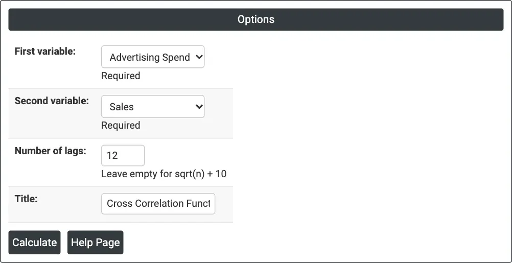
Figure 1 — Advertising Spend as the first variable and Sales as the second, with 12 lags each way.
Output Descriptions
- Cross Correlation Function (graph) — a bar for each lag from −k to +k with the dashed limits, and the note “Positive lag = <first variable> leads <second variable>”.
- Cross Correlation Function: <first variable>, <second variable> (table) — Lag and CCF.
- PDF export via Download.
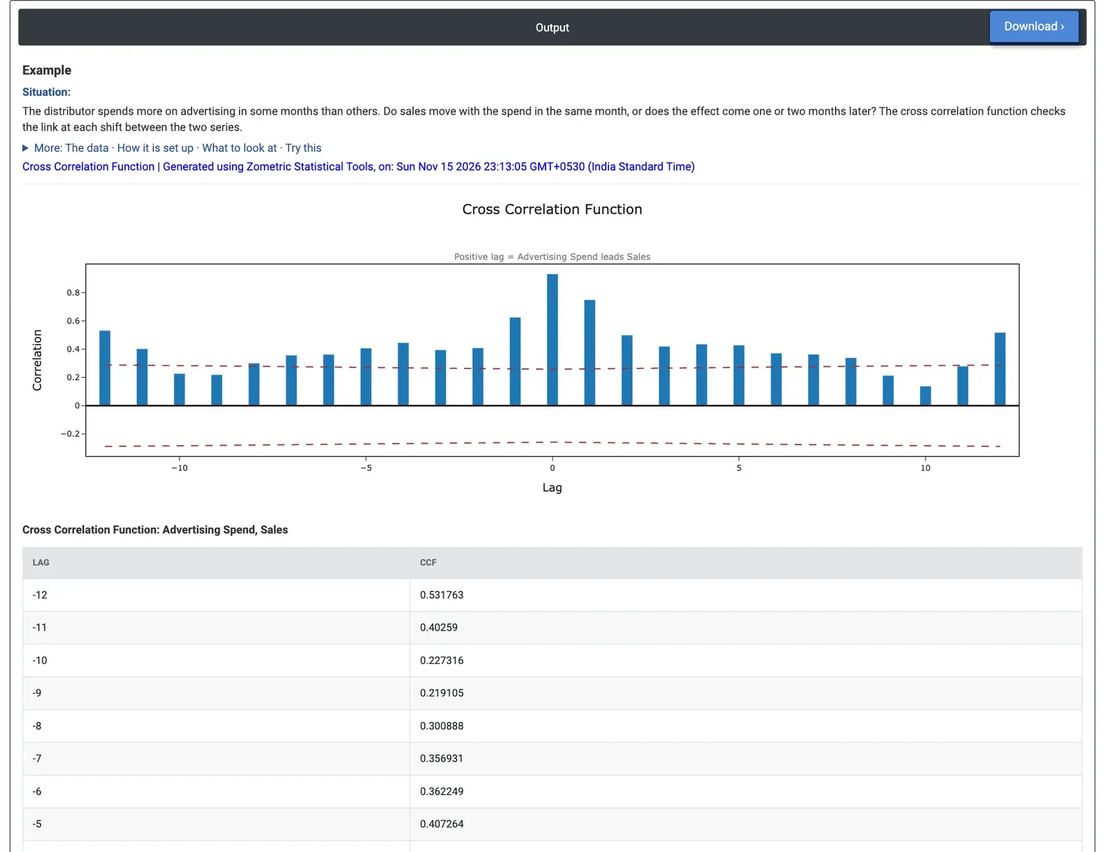
Figure 2 — Cross correlation of advertising spend with sales: the highest bar, 0.93, is at lag 0.
Worked Example
A consumer electronics distributor has 60 months of data (January 2020 to December 2024): units sold and advertising spend (thousand dollars) each month. Spend is higher in some months than others. The marketing manager asks whether sales respond in the same month or one or two months later. The analyst selects First variable = Advertising Spend, Second variable = Sales and Number of lags = 12.
The highest bar is at lag 0: 0.93. Sales move with spend in the same month. At lag +1 (spend one month before sales) the cross correlation is 0.75, and at lag −1 (sales one month before spend) 0.63. So there is no sign of an effect that builds up a month or two later: the link is strongest within the month. Most bars are above the limits (about ±0.26 to ±0.29); only lags −10, −9, +9, +10 and +11 fall inside. The values stay high as far out as 0.53 at lag −12 and 0.52 at lag +12 because both series share the upward trend and the year-end peak. These high values at every lag come from the common pattern, not from advertising working a year ahead.
For the decision this means modelling sales on same-month spend first; a lagged spend term adds little. If First variable and Second variable are swapped, the plot mirrors: lag +1 then reads 0.63 and lag −1 reads 0.75. To test a delayed effect in a regression, build last month's spend as a column with the Lag tool.