
Decomposition
On this page
Purpose
Decomposition splits a seasonal time series into a straight-line trend, a repeating seasonal pattern and what is left over. It answers questions such as “how much does demand grow each month?” and “how far above or below the trend is December, every year?”, and it forecasts by extending the trend and repeating the seasonal pattern. Use it for monthly, quarterly or shift-pattern data with a stable season, for example to plan capacity or stock for the peak months.
Key Capabilities
- Multiplicative model (each season is a percentage above or below the trend) or additive model (each season is a fixed amount above or below).
- Seasonal index for every period of the season and the fitted trend equation.
- Forecasts for any number of periods, from the end of the series or from an earlier row to test the method against known data.
- MAPE, MAD and MSD accuracy measures.
- Decomposition plot (observed, trend, seasonal, residual), Component Analysis and Seasonal Analysis graphs, and optional four-in-one residual plots.
- Full results table with trend, seasonal, detrended, seasonally adjusted, fitted and error values for each row.
Statistical Methods
The tool uses classical decomposition. First it smooths the data with a centred moving average of length L (the seasonal length); for an even L it uses the 2×L average, so each value sits on a time point. The raw seasonal values are the data divided by this average (multiplicative) or minus it (additive). For each period of the season the median of its raw values is taken, and the medians are scaled to average 1 (multiplicative) or 0 (additive): these are the seasonal indices.
The data are then seasonally adjusted (divided by, or minus, the index) and a least-squares straight line Yt = b₀ + b₁·t is fitted to the adjusted data. The fit for each row is trend × index (multiplicative) or trend + index (additive), and the error is data − fit for both models. Forecasts extend the trend line and apply the index of the matching period; no prediction intervals are given. With a forecast origin, indices and trend are recalculated from the data up to that row. Accuracy: MAPE = mean of |error / data| × 100, MAD = mean |error|, MSD = mean error².
The series needs at least two full seasons and no gaps; the multiplicative model needs all values above zero. Choose multiplicative when the seasonal swing grows with the level of the series, additive when it stays the same size.
Input Fields & Options
Field | Description |
Variable (Y) | Required. The numeric series, in time order. |
Seasonal length | Required, at least 2. Number of periods per season, e.g. 12 for monthly data with a yearly pattern, 4 for quarterly data. |
Model | Additive (default) or Multiplicative. |
First observation is in seasonal period | Default 1. The position of the first row in the season, e.g. 6 when the season starts in January and the data start in June. |
Number of forecasts | Default 0 (none), up to 1000. |
Forecast origin (row) | Optional, active when forecasts are requested. Forecasts start after this row and use the data up to it; blank = end of the series. |
Results to display | Summary table (default) or Summary table and results table. |
Residual plots (four in one) | Unticked by default. Normal probability plot, residuals versus fits, histogram and residuals versus order. |
Component analysis graph / Seasonal analysis graph | Both ticked by default. Add the two extra four-panel graphs. |
Title | Title of the output. Default Decomposition. |
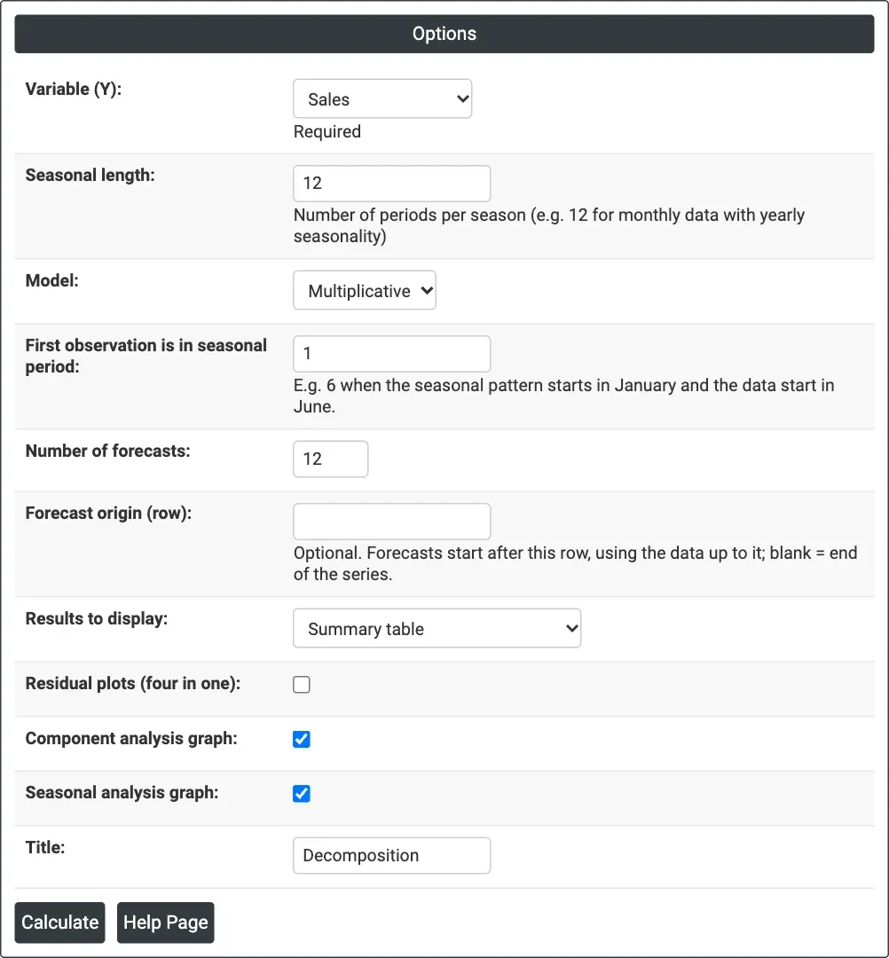
Figure 1 — Multiplicative decomposition of monthly Sales with a seasonal length of 12 and 12 forecasts.
Output Descriptions
- <Model> Decomposition of <variable> — four panels: Observed, Trend, Seasonal and Residual, with MAPE, MAD and MSD in the title.
- Component Analysis for <variable> — Original Data, Detrended Data, Seasonally Adjusted Data, and Seasonally Adj. and Detrended Data.
- Seasonal Analysis for <variable> — Seasonal Indices, Detrended Data by Season (box plots), Percent Variation by Season and Residuals by Season.
- Residual Plots for <variable> — when ticked.
- Method — model type, data column, length, seasonal length (and first period and forecast origin when set).
- Fitted Trend Equation, Seasonal Indices (one per period), Accuracy Measures (MAPE, MAD, MSD) and Forecasts (period and forecast).
- Results — when chosen: Period, data, Trend, Seasonal, Detrend, Deseason, Predict and Error for each row.
- PDF export via Download.
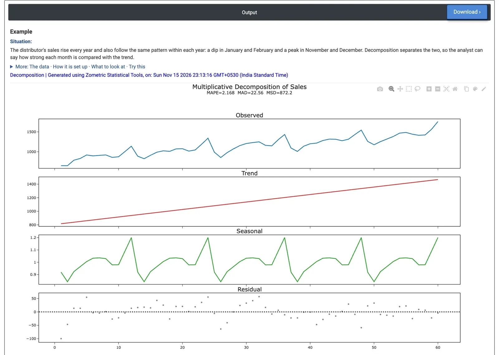
Figure 2 — Multiplicative decomposition of 60 months of sales: a rising trend, a seasonal pattern that repeats every year and small residuals.
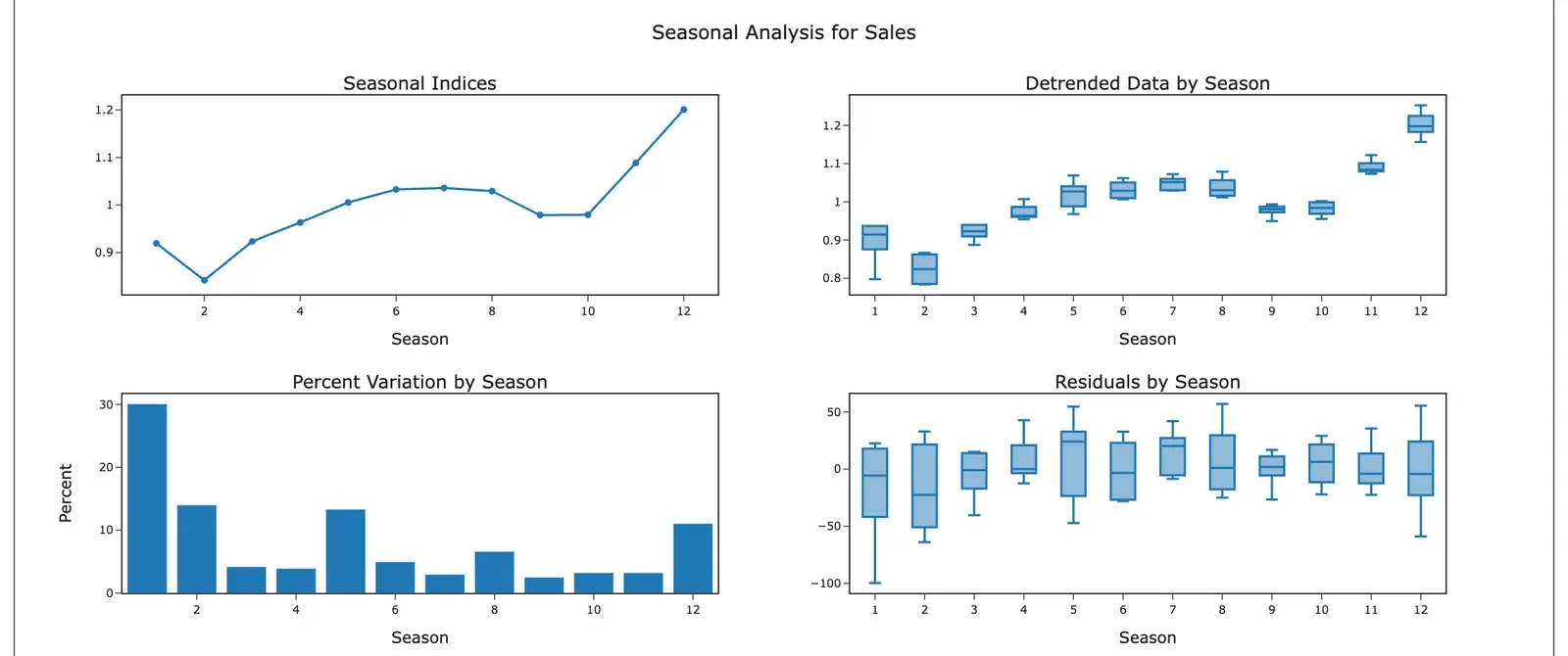
Figure 3 — Seasonal Analysis for the example: February is the lowest month (index 0.84) and December the highest (1.20).
Worked Example
A consumer electronics distributor's sales rise every year and also follow the same pattern within the year: a dip early in the year and a peak in November and December. The sales analyst has 60 months of unit sales (January 2020 to December 2024) and needs to know how strong each month is compared with the trend, and a forecast for 2025. The analyst selects Variable (Y) = Sales, Seasonal length = 12, Model = Multiplicative and Number of forecasts = 12.
The trend is Yt = 805.33 + 11.049×t: about 11 more units every month. The seasonal indices show December at 1.20 (20% above the trend) and November at 1.09, while February is at 0.84 (16% below the trend) and January and March at 0.92. MAPE is 2.2% (MAD 22.6 units), against 7.4% for a straight trend line alone on the Trend Analysis page: the season explains most of what the line misses. The 2025 forecasts follow the same shape, from 1,255 units in February to 1,922 in December.
For planning this means stock and staffing for December need to be about a fifth above the trend level, and February can run well below it. The Percent Variation by Season graph shows that January has the most variation from year to year, so its forecast is the least certain. With Model = Additive the MAPE is 2.21% against 2.17%, so either form describes this season; the additive version gives each month a fixed number of units (December +224, February −193) instead of a percentage.