
Differences
On this page
Purpose
Differences computes the change in a series from one period to another: each value minus the value a set number of rows (the lag) earlier. A lag of 1 gives the period-to-period change and removes a trend; a lag equal to the season (12 for monthly data, 4 for quarterly) compares each period with the same period a season before and removes the seasonal pattern. Use it to see whether growth is steady, and to make a series stationary before checking its autocorrelation or fitting an ARIMA model.
Key Capabilities
- Differences at any lag from 1 to 365.
- Plot of the differenced series against the row number, with a zero line.
- Table with the row number, the original value and the difference for every row; rows without an earlier value show *.
- Keeps gaps in place: a missing value gives a missing difference instead of shifting the later rows.
Statistical Methods
For a series y₁ … yₙ and lag k, the difference in row t is dₜ = yₜ − yₜ₋ₖ for t = k + 1 … n. The first k rows have no earlier value and are shown as *. A missing value anywhere in the series gives a missing difference in its own row and in the row k later. The series needs more than k values.
A first difference (k = 1) removes a straight-line trend: if yₜ grows by b units per period, the differences vary around b. A seasonal difference (k = the seasonal length) removes a stable seasonal pattern and leaves the change from one season to the next; for a series with a linear trend those differences vary around k × b. In ARIMA terms, a lag-1 difference is d = 1 and a seasonal difference is D = 1. Differencing the same series twice (for example lag 12 and then lag 1) needs the first result as a new column.
Input Fields & Options
Field | Description |
Variable | Required. The numeric column to difference, in time order. |
Lag | Required, 1 to 365, default 1. Number of rows between the two values subtracted. |
Title | Title shown on the graph. Default Differences. |
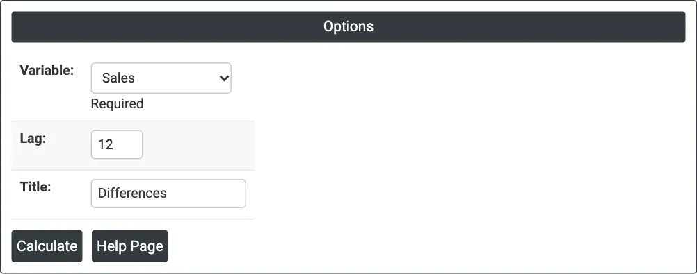
Figure 1 — Twelve-month differences of monthly Sales.
Output Descriptions
- Differences (graph) — the differenced values against the row index, with a dotted line at zero.
- Differences (table) — Row, the original column and Difference (lag k) for every row.
- PDF export via Download.
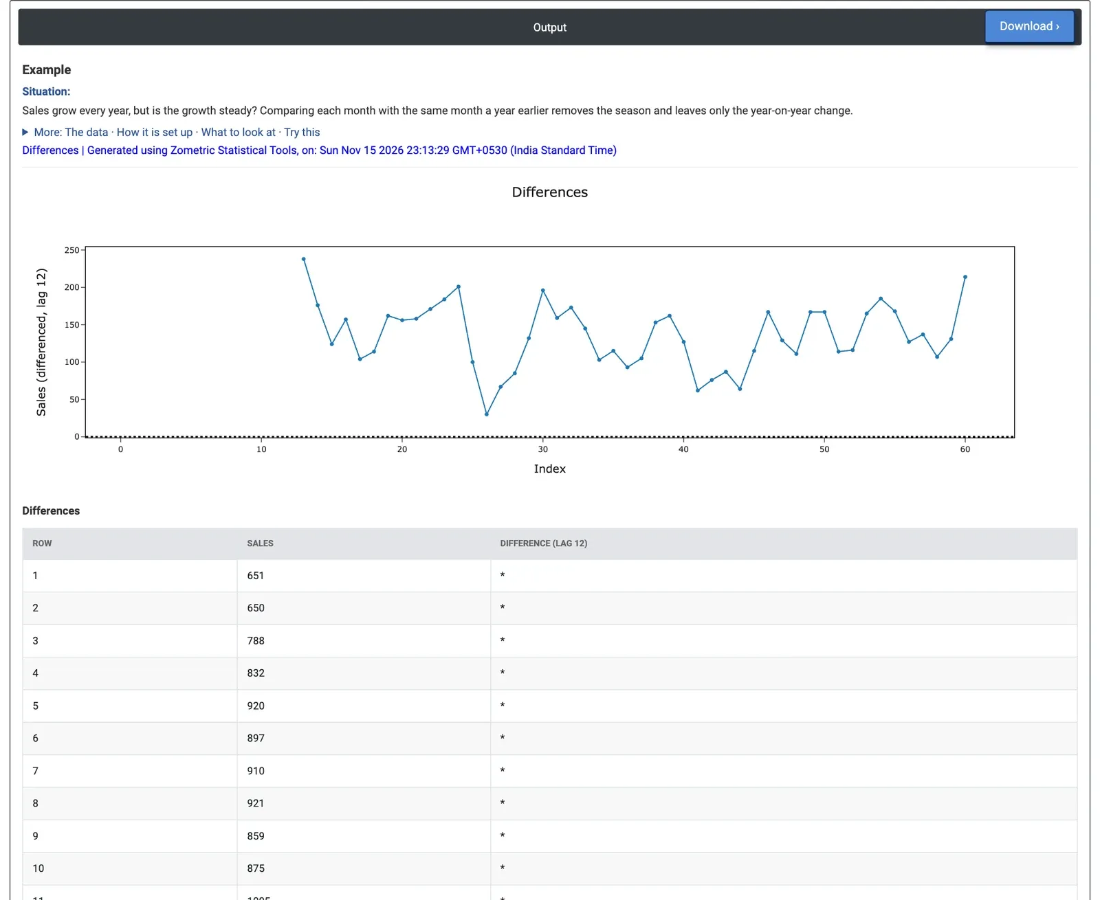
Figure 2 — Year-on-year change in monthly sales: every value is above zero, between +30 and +238 units.
Worked Example
A consumer electronics distributor's sales grow every year but also follow a yearly pattern, with a dip early in the year and a peak in December. The sales manager wants to know whether the growth is steady. The analyst takes 60 months of unit sales (January 2020 to December 2024), selects Variable = Sales and sets Lag = 12, so that each month is compared with the same month a year earlier and the season drops out.
The first 12 rows show * because there is no earlier year. All 48 year-on-year changes are positive: no month sold fewer units than the same month a year before. They range from +30 (February 2022) to +238 (January 2021), with an average of +135 units, about 11 a month, matching the trend line found by Decomposition (11.05 units a month). The average change by year was +162 in 2021, +117 in 2022, +113 in 2023 and +150 in 2024: growth slowed in 2022 and 2023 and picked up again in 2024.
With Lag = 1 the month-to-month changes swing from −352 (December 2021 to January 2022) to +195 (November to December 2024). The seasonal swings are so large that the growth (an average of +19 units a month) is hard to see, which is why the 12-month difference is the right choice for this series. The same 12-month difference is the seasonal differencing (D = 1) used in the ARIMA example.