
Distribution ID Plot (Right Censoring)
On this page
Purpose
Distribution ID Plot (Right Censoring) helps you choose a life distribution before you estimate reliability or percentiles. It fits six common distributions to the same failure-time data, including units that were removed or still running (right-censored), and draws a probability plot for each. The distribution whose points lie closest to a straight line fits best. Use it as the first step before Parametric Distribution Analysis or a Distribution Overview Plot.
Key Capabilities
- Fits Weibull, Lognormal, Exponential, Normal, Logistic and Loglogistic distributions in one run.
- Handles right-censored data through a censoring column and censoring value.
- Ranks the distributions by the correlation coefficient of their probability plots.
- One probability plot panel per distribution, with the fitted line, its confidence bounds and the failure points.
- Reports any distribution that could not be fitted to the data.
Statistical Methods
In the censoring column, rows equal to the censoring value are right-censored (the unit had not failed when it was last seen) and every other row is a failure. Each of the six distributions is fitted to all rows by maximum likelihood, in which a failure contributes its density f(t) and a censored unit contributes its survival probability S(t) = 1 − F(t).
The plotted points are the failure times with nonparametric estimates of the cumulative probability of failure from the Nelson-Aalen method, which accounts for the censored units at risk at each failure time. Each panel transforms the axes so that its distribution would plot as a straight line: the time axis is logarithmic for Weibull, Lognormal and Loglogistic, and linear for Normal, Logistic and Exponential, and the probability axis uses the matching scale (labelled in percent). The red line is the fitted distribution's cumulative distribution function on the same scale. Each panel also shows two-sided confidence bounds (dotted) at the Confidence level, as Minitab draws them: for each percent p, the percentile t_p of the fitted distribution with its variance by the delta method from the inverse Hessian of the log-likelihood, the interval formed on ln(t_p) for Weibull, Lognormal, Exponential and Loglogistic and on t_p for Normal and Logistic. Points well outside the bounds point to a poor fit.
The correlation coefficient for each panel is the Pearson correlation between the plotted x values (time, or ln(time) on a log axis) and the transformed probabilities of the failure points. Values close to 1 mean the points lie close to a straight line. Small differences between the top distributions do not prove that one fits better; look at the panels, especially the tails, and consider engineering knowledge, for example that Weibull is the usual choice for failure times.
Input Fields & Options
Field | Description |
Variable | Required. Time to failure, or time to censoring for units removed or still running. |
Use censoring column | Required. Rows equal to the censoring value are right-censored; every other row is a failure. Every row needs a value. |
Censoring value | The value in the censoring column that marks a censored unit. Default 0, so 1 = failure. |
Confidence level (%) | Default 95; 50 to 99.99. Sets the confidence bounds drawn around each fitted line. |
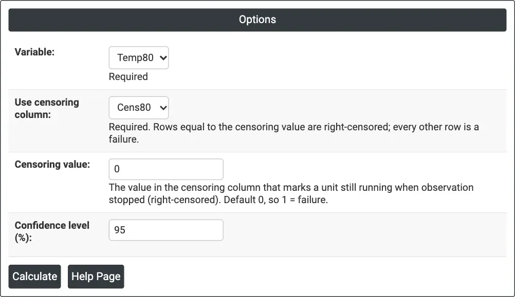
Figure 1 — Options for the example: winding test times at 80 °C (Temp80) with censoring column Cens80, censoring value 0.
Output Descriptions
- Correlation ranking — each distribution and its correlation coefficient, from best to worst.
- Messages — any distribution that could not be fitted, with the reason.
- Distribution ID Plot — one probability plot panel per distribution in ranking order, titled with its correlation (r), showing the failure points, the fitted line and its confidence bounds.
- PDF export via Download.
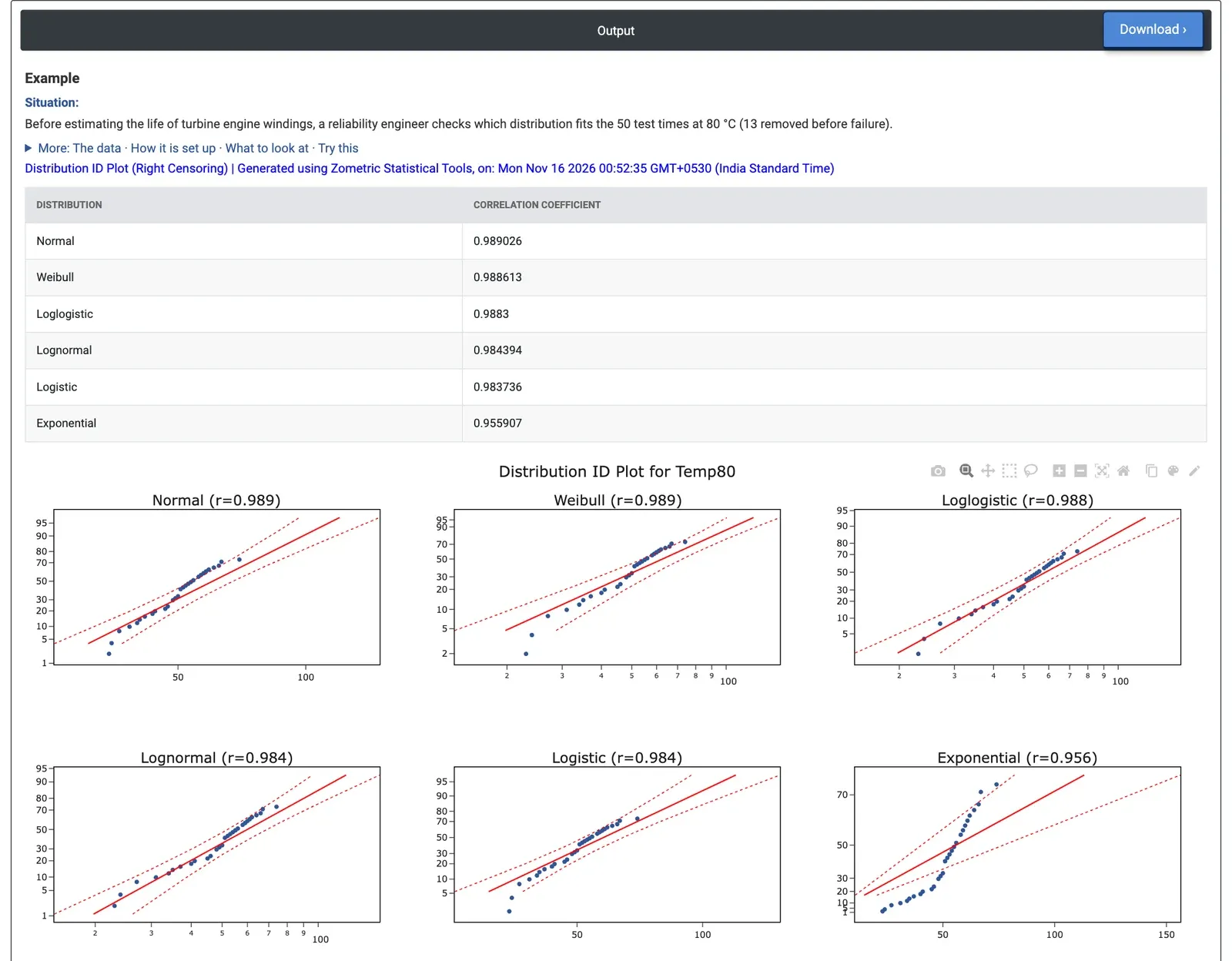
Figure 2 — Correlation ranking and probability plots for 50 winding test times: Normal, Weibull and Loglogistic are close to 0.989; Exponential is clearly worst at 0.956.
Worked Example
A reliability engineer tests 50 turbine engine windings at 80 °C. 37 fail during the test and 13 are removed before failure, so their times are censored. Before estimating life percentiles the engineer wants to know which distribution describes the data. The engineer sets Variable = Temp80, Use censoring column = Cens80 and Censoring value = 0, since Cens80 is 1 for a failure and 0 for a removed winding.
The correlation coefficients are Normal 0.9890, Weibull 0.9886, Loglogistic 0.9883, Lognormal 0.9844, Logistic 0.9837 and Exponential 0.9559. The top four are practically tied, so the data alone cannot choose between them. Exponential is clearly worst: its panel shows a strong curve, so the failure rate is not constant and a model that assumes random failures would mislead.
For the engineer, Weibull is a sensible choice: it fits as well as the others, it cannot give negative times, and its shape parameter shows whether failures are early, random or wear-out. Where the candidate distributions differ most is in the tails, so the engineer checks the panels at the low and high ends and, if extreme percentiles matter, compares the estimates from more than one distribution. The next step is a Distribution Overview Plot or Parametric Distribution Analysis with Weibull.