
Distribution Overview Plot (Arbitrary Censoring)
On this page
Purpose
Distribution Overview Plot (Arbitrary Censoring) fits one life distribution to failure data in which exact failure times are not always known, and shows the fit four ways on one page: a probability plot, the probability density function, the survival function and the hazard function. The data can mix exact failures with right-, left- and interval-censored units, as in inspection records where a failure is only found at the next check. Use it to check the chosen distribution and to see how the failure rate changes with age.
Key Capabilities
- Data entered as a Start column and an End column; the pattern of blank and filled cells sets the type of censoring on each row.
- Exact, right-, left- and interval-censored rows in the same data set.
- Six distributions: Weibull, Lognormal, Exponential, Normal, Logistic and Loglogistic.
- Maximum likelihood parameter estimates with standard errors, and the mean life.
- Probability plot with confidence bounds, and density, survival and hazard curves of the fitted distribution.
Statistical Methods
Each row is read from its Start and End values: Start = End is an exact failure; Start < End is an interval-censored failure between the two times; End blank is right-censored at Start; Start blank is left-censored at End. Every row needs at least one value, and Start must not be greater than End.
The chosen distribution is fitted by maximum likelihood: an exact failure contributes the density f(t), a right-censored unit 1 − F(Start), a left-censored unit F(End) and an interval-censored unit F(End) − F(Start). Standard errors come from the inverse of the Hessian of the log-likelihood at the estimate. Weibull is reported with scale Alpha (the time by which 63.2% fail) and shape Beta; Normal and Logistic with Mu and Sigma; Lognormal with Mu and Sigma of ln(time); Loglogistic with scale Alpha and shape Beta; Exponential with its failure rate Lambda. The mean is the mean life of the fitted distribution.
The probability plot shows nonparametric estimates of the cumulative probability of failure from the Turnbull method, which spreads each interval-censored failure over the times where it could have happened, on axes that make the chosen distribution a straight line, with the fitted line in red. The other panels show the density f(t), the survival function S(t) = 1 − F(t) and the hazard function h(t) = f(t) / S(t). A rising hazard means wear-out, a flat one random failures and a falling one early-life failures. The probability plot also shows two-sided confidence bounds (dotted) at the Confidence level, as Minitab draws them: confidence intervals for the percentiles t_p of the fitted distribution, from the delta method on the inverse Hessian, formed on ln(t_p) for Weibull, Lognormal, Exponential and Loglogistic and on t_p for Normal and Logistic.
Input Fields & Options
Field | Description |
Start column | Required. Last known good time, or the exact failure time. Leave Start blank on a row to mark it left-censored. |
End column | Required. First known failed time, or the exact failure time. Leave End blank on a row to mark it right-censored. Start = End means an exact failure; Start < End means interval-censored. Must be a different column from Start. |
Assumed distribution | Weibull (default), Lognormal, Exponential, Normal, Logistic or Loglogistic. |
Confidence level (%) | Default 95; 50 to 99.99. Sets the confidence bounds on the probability plot. |
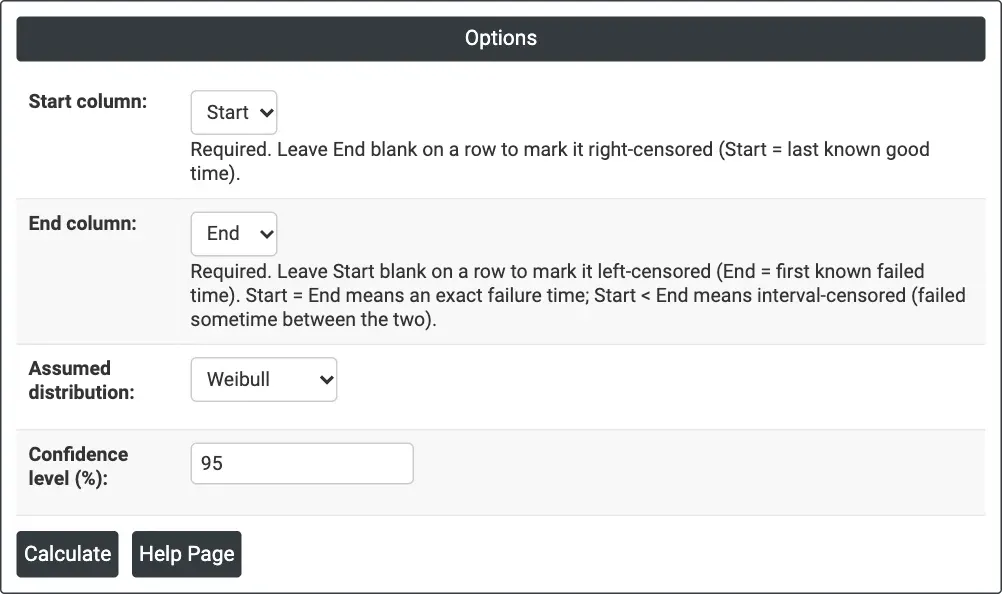
Figure 1 — Options for the example: inspection data in Start and End columns, Weibull distribution.
Output Descriptions
- Parameter estimates — Parameter, Estimate and Standard Error of the fitted distribution.
- Characteristics — the mean life of the fitted distribution.
- Distribution Overview Plot for Start-End — four panels: Probability Plot (with confidence bounds), Probability Density Function, Survival Function and Hazard Function.
- PDF export via Download.
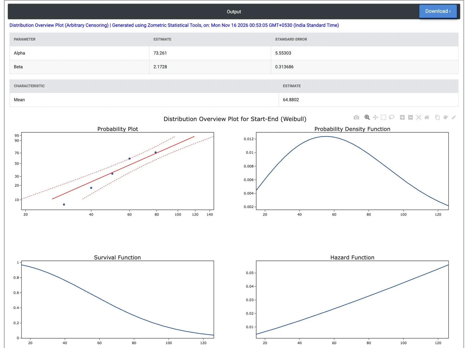
Figure 2 — Weibull overview for 50 windings checked every 10 hours: Alpha 73.3 h, Beta 2.17, mean 64.9 h, with a steadily rising hazard.
Worked Example
This example uses the 50 turbine engine windings tested at 80 °C from the Distribution Overview Plot (Right Censoring) page, recorded as they would be if the windings were only checked every 10 hours from 30 hours onwards. 4 windings found failed at the first inspection are left-censored (Start blank, End = 30), 33 found failed at later inspections are interval-censored (for example Start = 50, End = 60), and 13 removed before failure are right-censored at their removal times (End blank). The engineer selects Start and End as the Start and End columns and keeps Assumed distribution = Weibull.
The fitted Weibull has scale Alpha = 73.26 hours (standard error 5.55) and shape Beta = 2.173 (standard error 0.314), with a mean life of 64.88 hours. These are close to the values from the exact failure times (Alpha 73.34 hours, Beta 2.318), so the 10-hour inspection grid loses little information here, although the standard errors are slightly larger. The Survival Function gives 0.94 at 20 hours, 0.76 at 40 hours and 0.30 at 80 hours, and the median life is 61.9 hours. The 95% bounds on the probability plot give 18.8 to 36.0 hours for the 10th percentile (estimate 26.0 hours) and 53.0 to 72.3 hours for the median, slightly wider than from the exact times.
The probability plot has five points, at 30, 40, 50, 60 and 79 hours, where the Turnbull estimate places the failures, and they follow the fitted Weibull line, apart from the point at 30 hours, which sits a little below it. Because Beta is above 1, the Hazard Function rises with age, from about 0.0065 failures per hour at 20 hours to about 0.033 at 80 hours: the windings wear out. For the maintenance team, this supports planned replacement before the steep part of the curve. With Assumed distribution = Lognormal the mean life is 67.82 hours and the hazard levels off at about 0.03 per hour after 80 hours instead of rising, so the choice of distribution matters most for predictions at long times.