
Distribution Overview Plot (Right Censoring)
On this page
Purpose
Distribution Overview Plot (Right Censoring) fits one life distribution of your choice to failure-time data, including units removed or still running (right-censored), and shows it four ways on one page: a probability plot, the probability density function, the survival function and the hazard function. Use it to check how well the chosen distribution fits and to see at a glance how the failure rate changes with age, before a fuller Parametric Distribution Analysis.
Key Capabilities
- Six distributions: Weibull, Lognormal, Exponential, Normal, Logistic and Loglogistic.
- Handles right-censored data through a censoring column and censoring value.
- Maximum likelihood parameter estimates with standard errors, and the mean life.
- Probability plot of the failure points against the fitted line and its confidence bounds, to judge the fit.
- Density, survival and hazard curves of the fitted distribution.
Statistical Methods
In the censoring column, rows equal to the censoring value are right-censored and every other row is a failure. The chosen distribution is fitted by maximum likelihood, in which a failure contributes its density f(t) and a censored unit its survival probability S(t). Standard errors come from the inverse of the Hessian of the log-likelihood at the estimate. The Weibull distribution is reported with scale Alpha (the time by which 63.2% fail) and shape Beta; Normal and Logistic with location Mu and scale Sigma; Lognormal with Mu and Sigma of ln(time); Loglogistic with scale Alpha and shape Beta; Exponential with its failure rate Lambda. The mean is the mean life of the fitted distribution.
The probability plot shows the failure times against nonparametric estimates of the cumulative probability of failure (Nelson-Aalen method, which allows for the censored units), on axes transformed so that the chosen distribution plots as a straight line; the time axis is logarithmic for Weibull, Lognormal and Loglogistic. The red line is the fitted distribution. Points close to the line mean a good fit; a systematic curve means the distribution is wrong for these data. The probability plot also shows two-sided confidence bounds (dotted) at the Confidence level, as Minitab draws them: confidence intervals for the percentiles t_p of the fitted distribution, from the delta method on the inverse Hessian, formed on ln(t_p) for Weibull, Lognormal, Exponential and Loglogistic and on t_p for Normal and Logistic.
The other three panels show the fitted distribution: the density f(t), the survival function S(t) = 1 − F(t), the chance that a unit lasts beyond time t, and the hazard function h(t) = f(t) / S(t), the failure rate of units that have survived to t. A rising hazard means wear-out, a flat hazard random failures and a falling hazard early-life failures. For Weibull, a shape Beta above 1 gives a rising hazard.
Input Fields & Options
Field | Description |
Variable | Required. Time to failure, or time to censoring for units removed or still running. |
Use censoring column | Required. Rows equal to the censoring value are right-censored; every other row is a failure. Every row needs a value. |
Censoring value | The value in the censoring column that marks a censored unit. Default 0, so 1 = failure. |
Assumed distribution | Weibull (default), Lognormal, Exponential, Normal, Logistic or Loglogistic. |
Confidence level (%) | Default 95; 50 to 99.99. Sets the confidence bounds on the probability plot. |
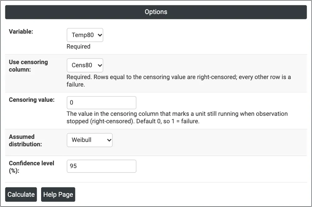
Figure 1 — Options for the example: winding test times at 80 °C (Temp80), censoring column Cens80 with censoring value 0, Weibull distribution.
Output Descriptions
- Parameter estimates — Parameter, Estimate and Standard Error of the fitted distribution.
- Characteristics — the mean life of the fitted distribution.
- Distribution Overview Plot — four panels: Probability Plot (with confidence bounds), Probability Density Function, Survival Function and Hazard Function.
- PDF export via Download.
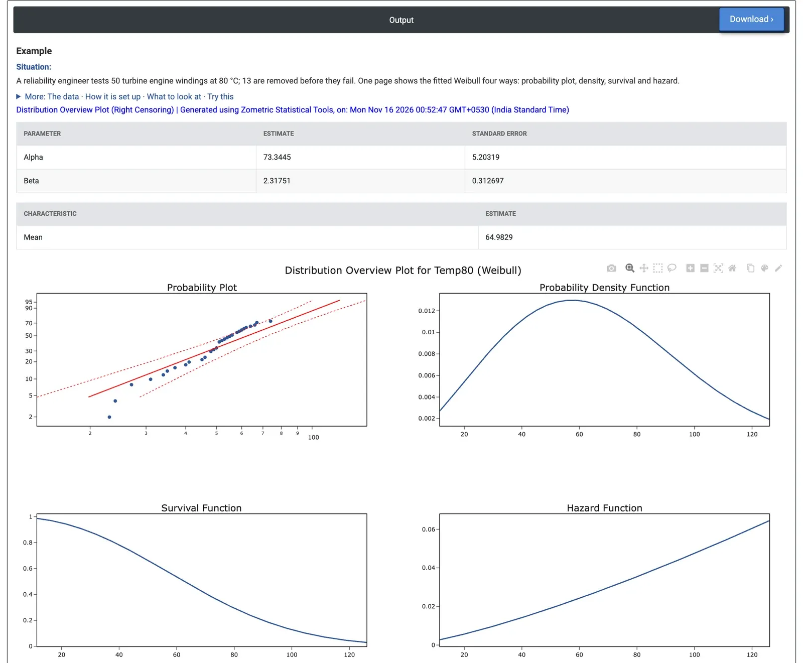
Figure 2 — Weibull overview for 50 winding test times: Alpha 73.3 h, Beta 2.32, mean 65.0 h, with a hazard that rises steadily with age.
Worked Example
A reliability engineer tests 50 turbine engine windings at 80 °C; 37 fail and 13 are removed before they fail. A Distribution ID Plot showed that Weibull fits about as well as any other distribution, so the engineer sets Variable = Temp80, Use censoring column = Cens80, Censoring value = 0 and Assumed distribution = Weibull.
The fitted Weibull has scale Alpha = 73.34 hours (standard error 5.20) and shape Beta = 2.318 (standard error 0.313), with a mean life of 64.98 hours. Because Beta is well above 1, the Hazard Function rises steadily with age, from about 0.006 failures per hour at 20 hours to about 0.035 at 80 hours: the windings wear out. The Survival Function gives 0.95 at 20 hours, 0.78 at 40 hours and 0.30 at 80 hours, and the median life is 62.6 hours. On the probability plot the 95% bounds give 20.8 to 37.1 hours for the 10th percentile (estimate 27.8 hours) and 54.2 to 72.4 hours for the median.
In the Probability Plot the points follow the line at the low end but sit above it between about 50 and 70 hours, so the engineer should treat extreme percentiles with care and compare with another distribution. With Assumed distribution = Normal, the fit gives Mu = 63.55 hours and Sigma = 27.55 hours. For maintenance, the rising hazard supports replacing windings on a schedule before they reach the steep part of the curve, rather than running them to failure.