
Empirical CDF
On this page
Purpose
The Empirical CDF plots, for every value of a measurement, the percentage of observations at or below it. The result is a step curve that shows the whole distribution at once: the median, the spread, the tails and any gaps. Use it to compare two or more groups (machines, suppliers, configurations) beyond their averages, to read off the share of parts below a limit, or to check the data against a fitted distribution.
Key Capabilities
- One step curve per variable, or per group of one variable when a By column is chosen.
- Several variables overlaid on one plot for a direct comparison.
- Optional fitted distribution overlaid as a dashed line: Normal, Lognormal, Weibull, Exponential, 2-Parameter Exponential, Smallest or Largest Extreme Value, Logistic or Loglogistic.
- Percent scale from 0 to 100 on the vertical axis, so percentiles can be read straight off the curve.
- Rows can be excluded or kept by row number or by a condition before plotting.
Statistical Methods
For each curve the non-blank numeric values are sorted, x₁ ≤ x₂ ≤ … ≤ xₙ, and the i-th value is plotted at the plotting position pᵢ = (i − 0.5) / n, shown as a percentage. The points are joined as a step (horizontal then vertical), so the curve rises by 100/n percent at each observation. The value where a curve crosses 50% is the median of that group; where it crosses 90% is the 90th percentile.
With a By column and a single variable, the rows are split by the levels of the By column and each level gets its own curve. With several variables, each variable gets a curve and the By column is ignored.
When a fitted distribution is chosen, its parameters are estimated separately for each curve (each group, or each variable), as in Minitab, and each fitted CDF is drawn over the range of its own data. The Normal uses the sample mean and standard deviation; the other distributions use maximum likelihood (Lognormal, Weibull, Exponential and Loglogistic with the threshold fixed at 0, so they need positive values). The legend shows the fitted parameters of each curve, so each group can be checked against its own model.
Input Fields & Options
Field | Description |
Variables | One or more numeric columns. Select one variable, or several to overlay their curves. |
By (grouping) column | Optional. One curve per level of this column. Only used when a single variable is selected. |
Overlay fitted distribution | Default “--- (empirical only)”: no fitted line. Or one of Normal, Lognormal, Weibull, Exponential, 2-Parameter Exponential, Smallest Extreme Value, Largest Extreme Value, Logistic, Loglogistic. |
Title | Title of the plot. Default “Empirical CDF”. |
Data Options: Subset (optional) | Exclude matching rows (default) or Include only matching rows; Row numbers (e.g. 3,7,12-15) and/or a Condition (e.g. Weight_kg > 100) select the rows. Has no effect when both are blank. |
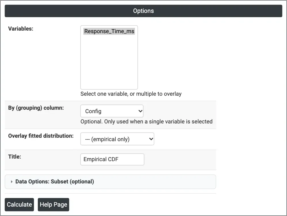
Figure 1 — Options for the example: Variables = Response_Time_ms, By (grouping) column = Config, no fitted distribution.
Output Descriptions
- Empirical CDF — step curve of percent against the variable for each group or variable, with markers at each observation and a legend naming the curves; the fitted distribution, if chosen, is a dashed line for each curve, in the curve's colour (black when there is only one curve), labelled with its parameters.
- PDF export via Download.
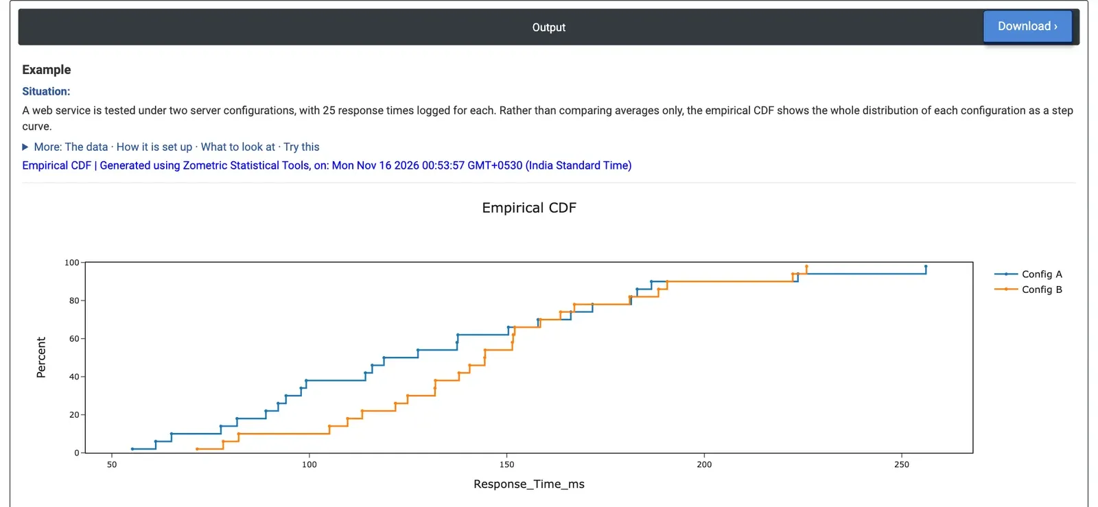
Figure 2 — Empirical CDF of response time for Config A (blue) and Config B (orange), 25 requests each.
Worked Example
An IT team tests a web service under two server configurations and logs 25 response times (ms) for each. The averages alone (129.7 ms for A, 143.6 ms for B) suggest A is faster, but the team wants to know how the whole distribution compares, especially the slow requests users notice. They select Response_Time_ms as the variable and Config as the By column, with no fitted distribution.
Reading across at 50%, the median is 118.9 ms for Config A and 144.4 ms for Config B: over most of the range B's curve lies to the right, so a typical request is slower on B. At 150 ms, 64% of A's requests are done against 56% of B's. At the top the curves cross: A's slowest request takes 256.1 ms against 225.9 ms for B's slowest, and A's spread is wider (standard deviation 51.8 against 39.7 ms). Both configurations have 92% of requests within 200 ms. So B is slower on a typical request while A has the longer tail; the choice depends on whether the median or the worst case matters more for the service.
Choosing Normal as the overlay adds a dashed normal curve for each configuration, fitted to its own 25 values: mean 129.7 ms and standard deviation 51.8 ms for A, mean 143.6 ms and standard deviation 39.7 ms for B. Where a step curve leaves its dashed curve, that configuration's response times are not normal.