
Fit Mixed Effects Model
On this page
Purpose
Fit Mixed Effects Model analyses a response that depends on two kinds of factor: fixed factors, whose particular levels you want to compare (two machines, three suppliers, a new and an old method), and random factors, whose levels are a sample from a larger population (batches, samples, operators, days). It tests the fixed factors and estimates how much variance each random factor adds. Use it when ignoring the random factors would make the fixed-factor tests too optimistic, for example when the same batches or parts are measured under every condition.
Key Capabilities
- One or more fixed categorical factors and continuous covariates, with one or more random factors.
- Variance components for each random factor and the error, with % of total, standard error, Z-test and confidence interval.
- F-tests of the fixed effects with Satterthwaite denominator degrees of freedom.
- Coefficients with Satterthwaite degrees of freedom, t-tests and confidence intervals.
- Model summary with S, R-sq, R-sq(adj), AICc, BIC and −2 log likelihood.
- Restricted maximum likelihood (REML) or maximum likelihood (ML) estimation.
- Data Options: subset the rows before the analysis.
Statistical Methods
The model is y = Xβ + Σ Zᵢuᵢ + ε, where Xβ holds the fixed factors (sum-to-zero −1/0/+1 coding) and covariates, each random factor i adds independent effects uᵢ with variance σᵢ², and the errors ε have variance σ². Random factors are independent variance components (no interactions are fitted). The variances are estimated by REML (default), which allows for the degrees of freedom used by the fixed effects and gives nearly unbiased variance components, or by ML, which is needed to compare models with different fixed effects by AICc or BIC. Rows with a missing value are dropped; every random factor needs at least 3 levels.
Given the variance estimates, the fixed coefficients are generalised least squares estimates. Each fixed term is tested with an F statistic whose denominator degrees of freedom come from the Satterthwaite approximation, and each coefficient with a t-test on Satterthwaite degrees of freedom. Variance components have standard errors from the Fisher information, a one-sided Z = Var / SE Var test that the component is zero, and a confidence interval calculated on the log scale, so it is never negative. With few levels of a random factor this Z-test has little power and the interval is wide.
R-sq compares the conditional fits (fixed effects plus predicted random effects) with the total variation. S is the square root of the error variance. AICc and BIC are smaller for better models; with REML they only compare models that have the same fixed effects.
Input Fields & Options
Field | Description |
Response (Y) | Numeric response column. Required. |
Fixed factors (categorical) | One or more columns whose specific levels are of direct interest. Required. |
Random factors (categorical) | One or more columns whose levels are a random sample from a larger population (e.g. Field, Batch, Operator), modelled as independent variance components. Required. |
Covariates (continuous) | Optional numeric columns, entered as fixed main effects only. |
Confidence level | Default 95. |
Estimation method | Restricted maximum likelihood (REML), the default, or Maximum likelihood (ML). |
Data Options: Subset (optional) | Exclude matching rows (default) or Include only matching rows, by row numbers and/or a condition. |
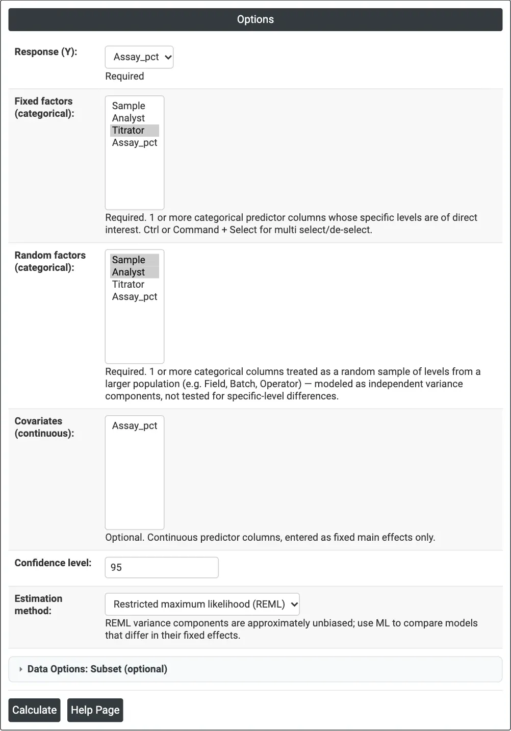
Figure 1 — Options for the titrator example: Assay_pct as the response, Titrator as a fixed factor, Sample and Analyst as random factors, REML.
Output Descriptions
- Method — variance estimation method and the degrees-of-freedom method for the fixed effects.
- Variance Components — Var, % of Total, SE Var, Z-Value, P-Value and confidence interval for each random factor, the error and the total.
- Tests of Fixed Effects — DF Num, DF Den, F-Value and P-Value for each fixed factor and covariate.
- Model Summary — S, R-sq, R-sq(adj), AICc, BIC and −2 log likelihood.
- Coefficients — Coef, SE Coef, DF, T-Value, P-Value and confidence interval.
- A warning is shown if the optimiser did not fully converge.
- PDF export via Download.
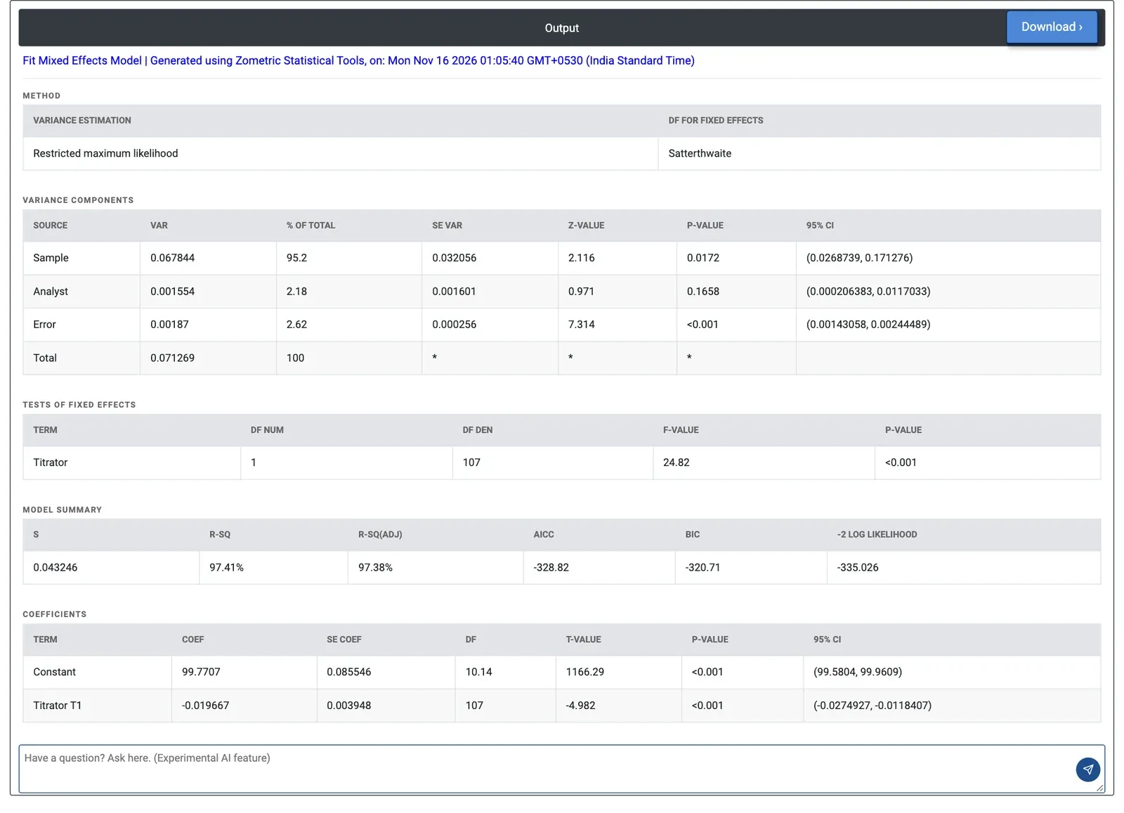
Figure 2 — Mixed model of the assay results: samples account for 95.2% of the variance, and the two titrators differ (F = 24.82, p < 0.001).
Worked Example
A soda ash lab measures product purity (Assay_pct) on two automatic titrators, T1 and T2. Ten samples are each measured twice by three analysts on both titrators: 120 results. The question is whether the two titrators give the same result. The titrators are the two instruments the lab owns, so Titrator is a fixed factor; the samples and analysts stand for many possible samples and analysts, so they are random factors. The lab enters Assay_pct as the response, Titrator as the fixed factor and Sample and Analyst as random factors, with REML. Load Example fills in these data (soda-ash-assay-expanded-grr, the same study as the Gage R&R Study (Expanded) example) and these settings.
The variance components show that the samples themselves differ most: 0.0678 (95.2% of the total, standard deviation about 0.26 percentage points). The analyst component is small, 0.00155 (2.18%), and not significantly different from zero (p = 0.1658); the error, the repeatability of a single result, is 0.00187 (standard deviation 0.043).
Titrator is significant: F = 24.82 on 1 and 107 degrees of freedom, p < 0.001. The coefficient for T1 is −0.0197 with sum-to-zero coding, so T2 reads about 0.039 percentage points higher than T1, close to one repeatability standard deviation. Because each sample was measured on both titrators, the sample-to-sample spread does not hide this difference. The lab decides to check the calibration of both titrators against a reference standard.