
Fully Nested ANOVA
On this page
Purpose
Fully Nested ANOVA splits the variation in a measurement into the levels of a hierarchy, such as batches, samples within each batch and repeat readings within each sample. Use it when each lower-level unit belongs to only one higher-level unit (Sample 1 of Batch 1 is not the same material as Sample 1 of Batch 2), and you want to know where most of the variation comes from, so you know where to act: the process, the sampling or the measurement.
Key Capabilities
- Two to four nested factors, from the outermost (e.g. Batch) to the innermost (e.g. Sample); repeat readings within the innermost factor form the error.
- One analysis per response when several responses are selected.
- ANOVA table with sequential sums of squares and F-tests of each level against the level below it.
- Variance components with their % of total and standard deviations.
- Expected mean squares, model summary and a table of means and standard deviations for every cell.
- Handles unbalanced data for the variance components; Data Options to subset the rows.
Statistical Methods
All factors are treated as random and each is nested in the one before it. The sum of squares for each factor is the spread of its cell means around the means of the level above; the error sum of squares is the spread of the readings around the innermost cell means. Each factor has (number of its cells − number of cells above) degrees of freedom, and the error has N − number of innermost cells.
Each factor is tested against the next factor inside it, and the innermost factor against the error: F = MS(factor) / MS(next inner term). F and P are given only for balanced designs (equal numbers of readings in every cell and equal numbers of sub-units in every unit); for unbalanced data the page says so and leaves them out.
The variance components come from the expected mean squares (ANOVA method): E(MS) of each factor is σ²(error) plus multiples of the components of that factor and the factors inside it, as shown in the Expected Mean Squares table, where (1), (2), … number the factors in nesting order and the last number is the error. Solving these equations from the innermost term outwards gives each component; a negative estimate is shown with 0% of the total. % of Total is each component's share of the summed variance, and StDev its square root. Rows with a missing response or factor value are dropped.
Input Fields & Options
Field | Description |
Responses | One or more numeric columns. Required; one analysis per response. |
Factor 1 (outermost) | The top level of the hierarchy, e.g. Batch. Required. |
Factor 2 (nested in Factor 1) | Required, e.g. Sample within Batch. |
Factor 3 (nested in Factor 2) / Factor 4 (nested in Factor 3) | Optional deeper levels; Factor 4 requires Factor 3. |
Data Options: Subset (optional) | Exclude matching rows (default) or Include only matching rows, by row numbers and/or a condition. |
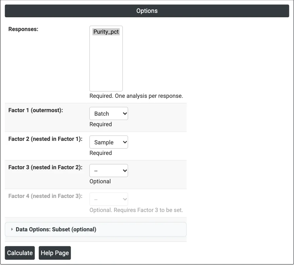
Figure 1 — Options for the purity example: Purity_pct as the response, Batch as Factor 1 and Sample (nested in Batch) as Factor 2.
Output Descriptions
- Analysis of Variance — DF, SS, MS, F and P for each factor, error and total.
- Variance Components — Var Comp, % of Total and StDev for each factor, error and total.
- Expected Mean Squares — the make-up of each mean square in terms of the variance components.
- Model Summary — S, R-sq and R-sq(adj).
- Means — N, mean and standard deviation of every innermost cell.
- PDF export via Download.
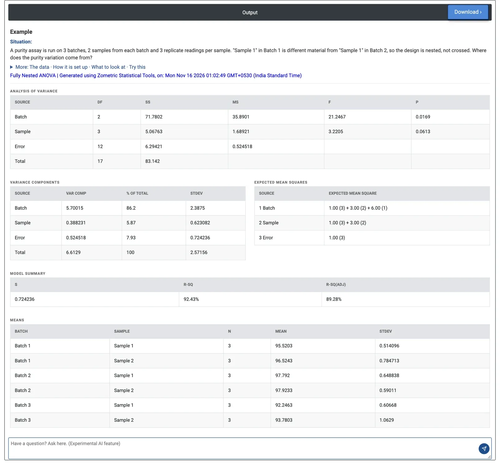
Figure 2 — Nested ANOVA of purity: batch-to-batch variation is 86.2% of the total; samples within a batch add 5.87% and repeat readings 7.93%.
Worked Example
A purity assay is run on 3 batches, with 2 samples taken from each batch and 3 repeat readings on each sample: 18 results. The quality team wants to know whether the spread in purity comes from the batch process, from the sampling or from the measurement. They select Purity_pct as the response, Batch as Factor 1 and Sample as Factor 2; the repeat readings form the error.
The batches differ: F = 21.25 on 2 and 3 degrees of freedom, p = 0.0169 (Batch is tested against Sample within Batch). Samples within a batch do not differ significantly at the 5% level (F = 3.22, p = 0.0613). Batch 3 runs lowest (cell means 92.25% and 93.78%) and Batch 2 highest (97.79% and 97.92%).
The variance components make the picture clear: batch-to-batch variance is 5.70 (86.2% of the total, standard deviation 2.39 percentage points), sample-to-sample 0.388 (5.87%) and the repeat readings 0.525 (7.93%, standard deviation 0.72). Better sampling or a more precise assay would change little; the team should look at what differs between batches.