
General Linear Model
On this page
Purpose
General Linear Model (GLM) runs an analysis of variance with one or more categorical factors, their two-way interactions and continuous covariates in one model. Use it when a one-way ANOVA is not enough: for example, when yield may depend on the machine, the operator, how the two combine, and also on a measured condition such as temperature, or when the data are unbalanced. It also covers the classic two-way ANOVA.
Key Capabilities
- Any number of fixed categorical factors, with all two-way factor interactions on request.
- Continuous covariates entered as main effects (analysis of covariance).
- Adjusted (Type III) or sequential (Type I) sums of squares; correct tests for unbalanced data.
- Least-squares means for each factor, adjusted for the other terms.
- Multiple comparisons of one factor's least-squares means by Tukey, Fisher, Bonferroni, Sidak or Dunnett (against a control), with grouping letters and an interval plot of the differences.
- Coefficients with VIF, model summary with R-sq(pred), unusual observations and four residual plots.
- Data Options: subset the rows before the analysis.
Statistical Methods
The model is fitted by ordinary least squares. Factors use sum-to-zero (−1, 0, +1) coding, so each coefficient is a level's deviation from the overall mean and the Type III test of a main effect averages over the levels of the other factors. Rows with a missing value in any selected column are dropped. Each term is tested with F = Adj MS(term) / MS(Error) on its own and the error degrees of freedom; with sequential sums of squares each term is tested after the terms above it. The Total row is the total sum of squares about the mean, which the adjusted sums of squares need not add up to with unbalanced data.
S = √MS(Error). R-sq(pred) = 1 − PRESS / SS Total, where PRESS sums the squared leave-one-out prediction errors. A least-squares mean is the model's prediction for a factor level with the other factors averaged over their levels and covariates at their mean; unlike raw means, it is not biased by unequal group sizes or covariate differences.
Comparisons use the difference between least-squares means with its standard error from the coefficient covariance matrix. Tukey uses the studentised range distribution for all pairs; Fisher uses individual t-tests; Bonferroni and Sidak adjust the t critical value for the number of pairs; Dunnett compares every level with a control using the multivariate t distribution. An interval that does not contain zero, or means that do not share a grouping letter, indicate a significant difference. Standardised residuals beyond ±2 are flagged R and leverages above 3p/n are flagged X. The model assumes independent, normally distributed errors with constant variance: check the residual plots.
Input Fields & Options
Field | Description |
Response (Y) | Numeric response column. Required. |
Factors (categorical) | One or more categorical predictor columns. Required. |
Covariates (continuous) | Optional numeric columns, entered as main effects only (no interactions with factors). |
Include all 2-way factor interactions | Ticked by default: adds every two-factor interaction. |
Confidence level | Default 95; used for the comparisons. |
Comparison procedure | None (default), Tukey, Fisher, Bonferroni, Sidak or Dunnett (vs. a control level). |
Comparison factor | Which factor's least-squares means are compared; required if a procedure is chosen. |
Control group level (Dunnett) | Control level for Dunnett; blank uses the first level. |
Grouping information / Interval plot for differences of means | Ticked by default: grouping letters table and plot of the comparison intervals. |
Sum of squares for tests | Adjusted (Type III, default) or Sequential (Type I). |
Residual versus fit graph / Residual versus order graph / Histogram / Probability plot | Residual plots; all ticked by default. |
Data Options: Subset (optional) | Exclude matching rows (default) or Include only matching rows, by row numbers (e.g. 3,7,12-15) and/or a condition (e.g. Temperature_C > 185). |
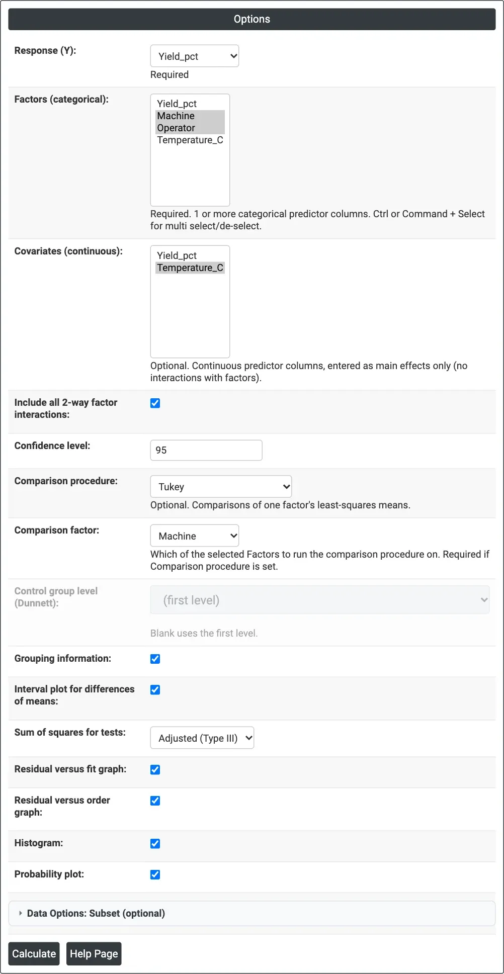
Figure 1 — Options for the yield example: Yield_pct with factors Machine and Operator, their interaction, covariate Temperature_C and Tukey comparisons of the machines.
Output Descriptions
- Method — factor coding and type of sums of squares.
- Factor Information — type, number of levels and level values of each factor.
- Analysis of Variance — DF, Adj SS (or Seq SS), Adj MS, F-Value and P-Value for each term, error and total.
- Model Summary — S, R-sq, R-sq(adj) and R-sq(pred).
- Least-Squares Means — N and LS mean of each level of each factor.
- Coefficients — Coef, SE Coef, T-Value, P-Value and VIF.
- Fits and Diagnostics for Unusual Observations — shown only when there are any.
- Grouping Information, Simultaneous (or Individual) Tests for Differences of Means and the interval plot — when a comparison procedure is chosen.
- Versus Fit, Versus Order, Residuals Histogram and Probability Plot.
- PDF export via Download.
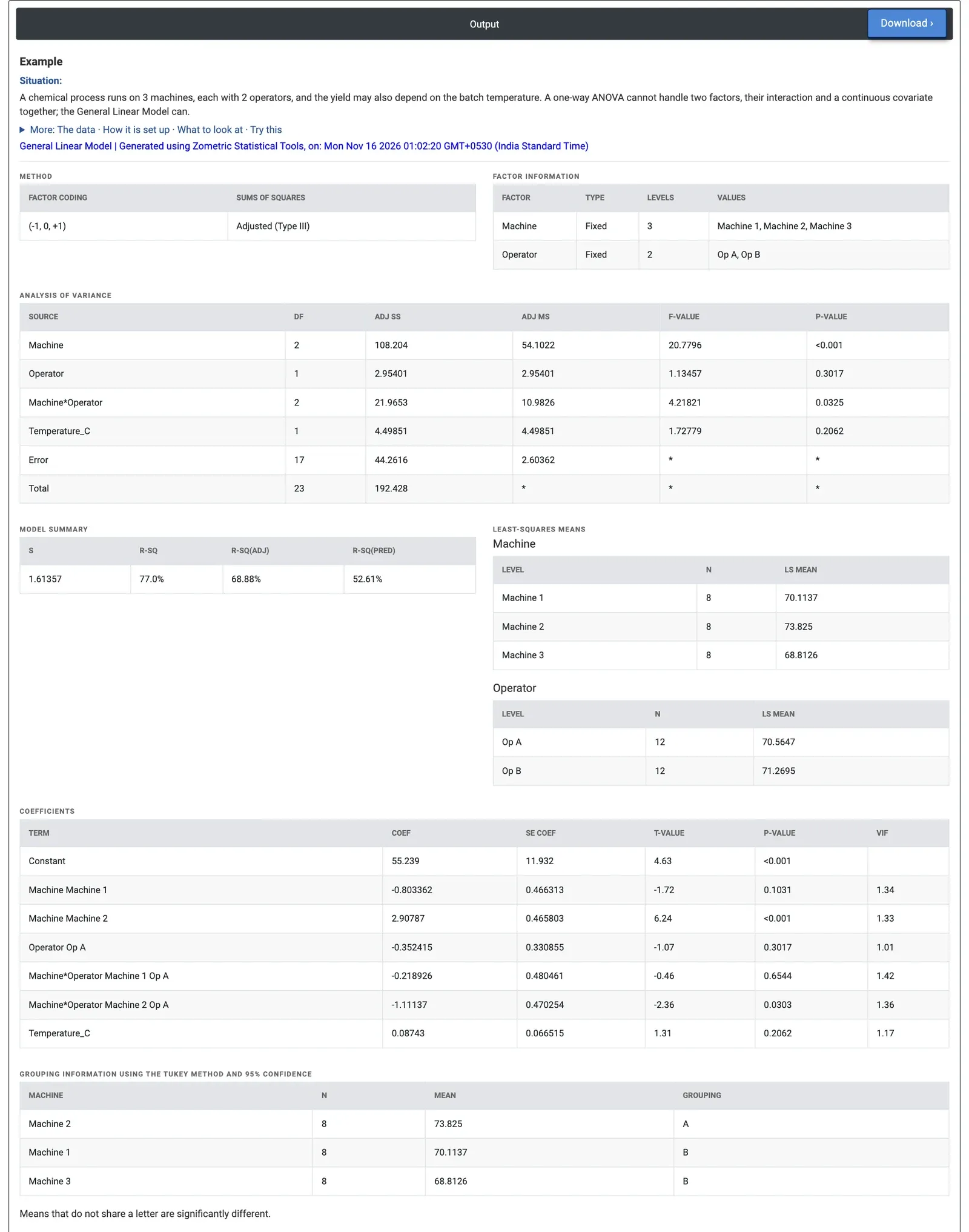
Figure 2 — GLM results for yield: Machine is significant (p < 0.001), so is the Machine*Operator interaction (p = 0.0325); Machine 2 has the highest LS mean, 73.83%.
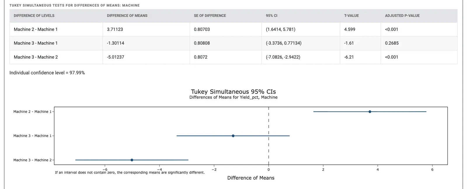
Figure 3 — Tukey comparisons of the machines: Machine 2 differs from both others; the interval for Machine 3 − Machine 1 contains zero.
Worked Example
A chemical process runs on three machines, each with two operators (Op A and Op B), and the batch yield may also depend on the batch temperature (170 to 190 °C). There are 24 batches, four for each machine and operator. The engineer selects Yield_pct as the response, Machine and Operator as factors with their interaction, Temperature_C as a covariate, and asks for Tukey comparisons of the machines.
The machines differ clearly (F = 20.78, p < 0.001). The Machine*Operator interaction is also significant (F = 4.22, p = 0.0325): Op B gets more from Machines 1 and 2, but less from Machine 3. Operator on its own (p = 0.3017) and temperature (p = 0.2062) have no significant effect over the range studied. The model explains 77.0% of the variation (R-sq(adj) 68.88%), with S = 1.61 percentage points; R-sq(pred) is lower at 52.61%, so predictions for new batches will be less precise than the fit suggests.
The least-squares means are 73.83% for Machine 2, 70.11% for Machine 1 and 68.81% for Machine 3. Tukey puts Machine 2 in group A on its own: it yields 3.71 points more than Machine 1 (95% CI 1.64 to 5.78) and 5.01 more than Machine 3, both with adjusted p < 0.001, while Machines 1 and 3 do not differ (adjusted p = 0.2685). The engineer studies what is different on Machine 2 and, because of the interaction, looks at the operator pairing on Machine 3 before standardising the method.