
Individual Value Plot
On this page
Purpose
The Individual Value Plot shows every observation as a dot, one column of dots per group. It suits small samples, where a boxplot or histogram summarises too much: you see each result, how the groups compare in centre and spread, and any single value that stands apart. Use it to compare machines, stations, shifts or suppliers before a formal test such as One-Way ANOVA.
Key Capabilities
- One Y variable, or several Y variables side by side (Multiple Y's).
- Optional grouping column on the X axis and a colour-category column for a second grouping.
- Group means joined by a line, to compare centres at a glance.
- Optional overlays: a boxplot behind the dots, or an interval bar showing each group mean with its 95% confidence interval.
- Adjustable horizontal jitter, so tied or close values do not hide each other.
- Optional exclusion of outliers by the 1.5×IQR rule, judged within each group.
- Optional guided interpretation: summary statistics per group and a report card with sample size, outlier and next-step checks.
Statistical Methods
The plot itself makes no estimate: every non-blank numeric value is drawn at its group's position, spread sideways by a random jitter (0 to 1, default 0.15) only to separate overlapping points. With several Y variables the columns are stacked into one, and each variable becomes a group on the X axis (or a colour when an X column is also set).
The mean line joins the arithmetic mean of each group. The interval bar is the mean ± t₀.₉₇₅,ₙ₋₁ × s / √n for each group, where s is the group's own sample standard deviation and n its size: a 95% confidence interval for the group mean. Bars that barely overlap suggest the means differ; a test such as One-Way ANOVA settles it.
Exclude outliers removes points below Q1 − 1.5×IQR or above Q3 + 1.5×IQR, with the quartiles and IQR worked out separately for each X and colour group (and each Y variable). The output then states how many points were excluded. The guided interpretation marks unusual points by the same 1.5×IQR rule, reports N, mean, standard deviation, minimum and maximum per group, and comments on sample size (at least 10, preferably 20 per group) and on whether the means and standard deviations appear to differ.
Input Fields & Options
Field | Description |
Y variable(s) | Required. One numeric column, or several (Ctrl/Cmd to select) to plot them side by side. |
X-axis (grouping) column | Optional. Categorical column; one column of dots per level. |
Color-category column | Optional. Second grouping shown by colour. Default “--” (none). |
Connect group means with a line | Joins the group means. Off by default. |
Overlay boxplot | Draws a grey boxplot behind the dots. Off by default. |
Overlay interval bar (mean +/- 95% CI) | Draws each group mean with its 95% confidence interval. Off by default. |
Jitter (0-1) | Horizontal spread of the dots. Default 0.15. |
Title | Title of the plot. Default “Individual Value Plot”. |
Discrete color sequence | Colour palette for the groups. Default D3. |
Exclude outliers (1.5×IQR rule) | Drops points beyond Q1 − 1.5×IQR or Q3 + 1.5×IQR within each group before plotting. Off by default. |
Data Options: Subset (optional) | Exclude matching rows (default) or Include only matching rows; Row numbers (e.g. 3,7,12-15) and/or a Condition (e.g. Station == "Station A") select the rows. |
Show guided interpretation | Adds a Summary Report, Diagnostic Report and Report Card that explain the result and check the data. Off by default. |
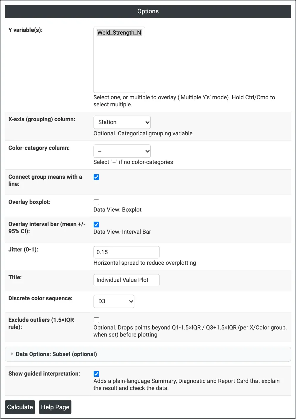
Figure 1 — Options for the example: Weld_Strength_N by Station, with group means joined, the 95% interval bar and the guided interpretation ticked.
Output Descriptions
- Individual Value Plot — the dots for each group, with the mean line, boxplot and interval bars when chosen.
- Note of excluded outliers — how many points the 1.5×IQR rule removed, when that option is ticked.
- Summary Report — a plot of the data by group and a table of N, Mean, StDev, Minimum and Maximum per group (guided interpretation only).
- Diagnostic Report — what to compare across groups: centre and variability (guided interpretation only).
- Report Card — checks on sample size and outliers, and next steps based on whether the means and standard deviations appear to differ (guided interpretation only).
- PDF export via Download.
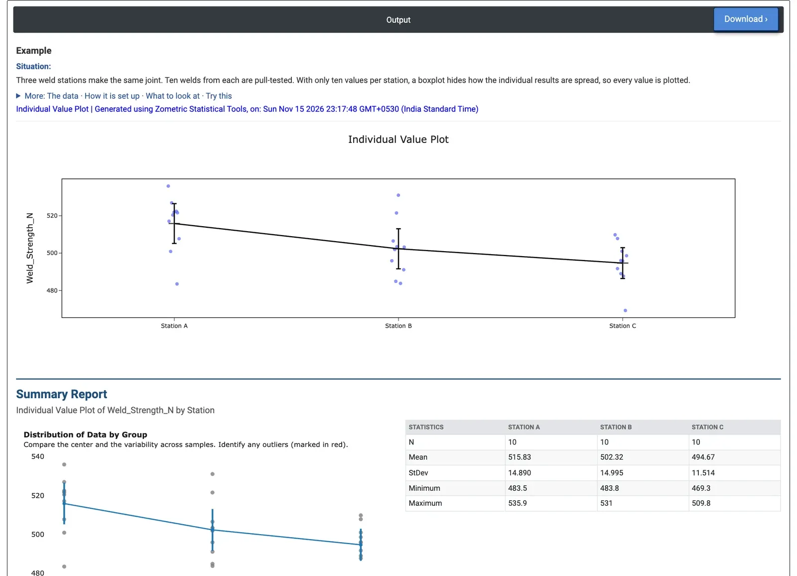
Figure 2 — Pull strength of ten welds from each of three stations, with group means joined and 95% confidence intervals, followed by the start of the Summary Report.
Worked Example
Three weld stations make the same joint, and ten welds from each are pull-tested. With only ten results per station, the engineer wants to see every value rather than a summary. Y variable(s) = Weld_Strength_N, X-axis (grouping) column = Station, with Connect group means with a line, Overlay interval bar and Show guided interpretation ticked.
The mean pull strength is 515.83 N at Station A, 502.32 N at Station B and 494.67 N at Station C, and the mean line falls steadily from A to C. The 95% interval for Station A (about 505.2 to 526.5 N) does not overlap Station C's (about 486.4 to 502.9 N), so C is likely weaker than A. The spreads are similar (standard deviations 14.9, 15.0 and 11.5 N), and the Report Card finds no outliers and notes that the means appear to differ while the standard deviations do not. Station C's lowest weld, 469.3 N, sits below the rest of its group but is not flagged.
The next step is a formal test: One-Way ANOVA on the same two columns gives p = 0.007, confirming that the stations differ. The team would then look at what is different about Station C (settings, electrode wear, operator) before its welds fall short of the strength requirement.