
Marginal Plot
On this page
Purpose
The Marginal Plot is a scatterplot of two variables with a small distribution plot along each axis. In one view it shows how Y moves with X and how each variable is distributed on its own: skewness, clusters, outliers and where most of the data lie. Use it when you study a relationship between two measurements and also need to know whether either one is unusual in shape, for example before a regression or when deciding whether a quick measurement can stand in for a slow one.
Key Capabilities
- Scatterplot of Y against X with a marginal plot on the top (X) and right (Y) edges.
- Four marginal types, applied to both axes: Histogram, Boxplot, Violin or Dot plot (rug).
- Optional category column: points and marginal plots are coloured by group, with a legend.
- Choice of colour palette.
- Interactive plot: zoom, pan and hover to read individual points.
Statistical Methods
The tool draws the data as they are; it fits no model and computes no test. Each row with both X and Y gives one point. The marginal plots summarise each variable separately: the histogram counts observations in equal-width bins chosen automatically; the boxplot shows the median, the quartiles (the box holds the middle 50% of the data) and whiskers; the violin adds a smoothed density outline to the box; the rug draws one tick per observation.
With a category column, each group gets its own colour in the scatterplot and its own marginal histogram, box, violin or rug, so you can see whether the groups differ in X, in Y or in both. The histograms of the groups are overlaid, and their heights are counts within each group.
To put a number on the relationship, use Correlation or Fitted Line Plot; the marginal plot is for seeing the pattern and the shape of each variable, and for spotting points that lie away from the rest.
Input Fields & Options
Field | Description |
X-axis column | Required. Numeric column on the horizontal axis. |
Y-axis column | Required. Numeric column on the vertical axis. |
Categorise based on column | Optional. Column whose values colour the points and marginal plots. Select “--” for no categories. |
Marginal plot type | Histogram (default), Boxplot, Violin or Dot plot (rug). Applied to both the X and Y margins. |
Title | Title of the plot. Default “Marginal Plot”. |
Discrete color sequence | Colour palette for the categories. Default D3. |
Data Options: Subset (optional) | Exclude matching rows (default) or Include only matching rows; Row numbers (e.g. 3,7,12-15) and/or a Condition (e.g. Activity == "low") select the rows. |
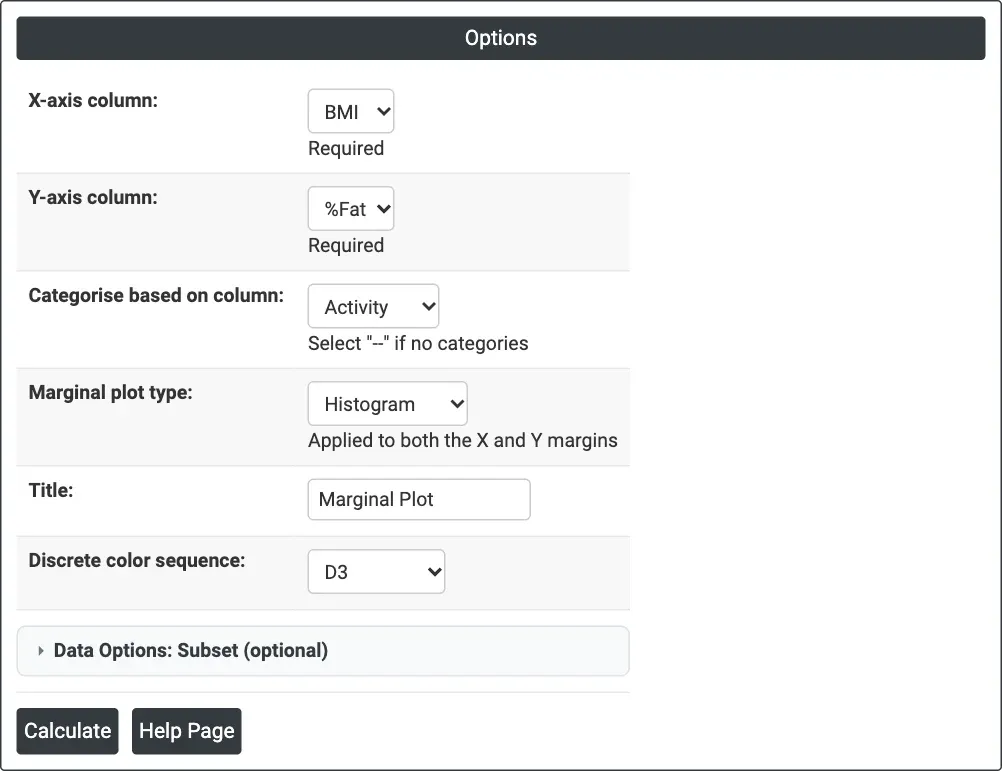
Figure 1 — Options for the example: X = BMI, Y = %Fat, categorised by Activity, histogram margins.
Output Descriptions
- Marginal Plot — scatterplot of Y against X, with the chosen marginal plot of X along the top and of Y along the right edge, coloured by category when one is chosen, with a legend.
- PDF export via Download.
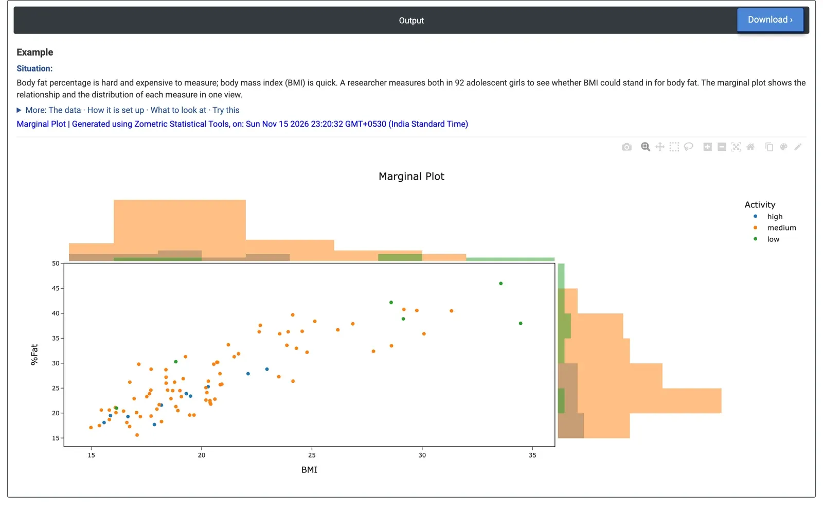
Figure 2 — Body fat percentage against BMI for 92 adolescent girls, coloured by activity level, with histograms of each variable on the margins.
Worked Example
Body fat percentage is slow and expensive to measure; body mass index (BMI) is quick. A researcher measures both in 92 adolescent girls, together with their physical activity level (low, medium, high), to see whether BMI could stand in for body fat. X-axis column = BMI, Y-axis column = %Fat, Categorise based on column = Activity, Marginal plot type = Histogram.
The points rise together: higher BMI goes with higher body fat (correlation 0.86, computed from the data). The spread widens at the top: for the 13 girls with BMI above 25, body fat ranges from 32.4% to 46%. The top histogram shows BMI skewed to the right, with most girls between 15 and 23 (median 19.5) and a few above 30; %Fat is also right-skewed (median 25.5%, maximum 46%).
The colours add a pattern the plain scatterplot hides: the 6 low-activity girls sit at the top right (mean BMI 26.8, mean body fat 36.1%), the 10 high-activity girls at the bottom left (mean BMI 18.8, mean body fat 22.6%), and the 76 medium-activity girls cover the range in between. So BMI is a useful first indicator of body fat, but not a precise replacement at high BMI, and activity level is worth recording alongside it. Changing Marginal plot type to Boxplot gives a compact summary of each axis per activity group instead of histograms.