
Matrix Plot
On this page
Purpose
The Matrix Plot draws a scatterplot for every pair of variables in one grid, so you can see at a glance which variables move together, which move in opposite directions and which are unrelated. Use it to screen several process inputs and outputs before a regression, to find variables that carry the same information, or to spot clusters and unusual points that a single scatterplot would miss.
Key Capabilities
- All-pairs matrix of two or more numeric variables: a scatterplot for each pair.
- Y-vs-X grid: one row per Y variable and one column per X variable, when X variables are set.
- Full matrix, or the lower-left or upper-right half only, to remove the duplicate panels.
- Optional colour category, to see whether groups (batch type, supplier, shift) separate.
- Optional guided interpretation: a Scatterplot Screener that ranks the other variables by how well each predicts the first one.
Statistical Methods
Only rows where all the selected variables are numeric are used, so every panel shows the same set of observations. The panel in row i and column j plots variable i (vertical) against variable j (horizontal). The plot itself fits nothing; a straight, narrow band of points means a strong linear relationship, a fan shape means unequal variation, and separate clouds mean clusters or stratification.
The guided interpretation takes the first selected variable as Y and each of the others as X (or the X variables, when set). For each X it fits a straight line and a quadratic by least squares and keeps the quadratic only if its squared term is significant at the 5% level. It reports the adjusted R² of the better model as the Predictive Ability: the share of the variation in Y that X alone explains, corrected for the number of terms. Each X is judged on its own; when inputs are correlated with each other, multiple regression is needed to see their joint effect.
Input Fields & Options
Field | Description |
Variables (or Y variables) | Required. Two or more numeric columns for an all-pairs matrix. If X variables is also set, these become the rows (Y variables) of a Y-vs-X grid. |
X variables (optional) | Optional. Builds a Y-variables-vs-X-variables grid (rows = Variables above, columns = this list) instead of an all-pairs matrix. |
Color-category column | Optional. Colours the points by group. Select “--” for no categories. |
Matrix layout | Full matrix (default), Lower left only or Upper right only. Only applies to the all-pairs matrix. |
Show histograms on the diagonal | Ticked by default: draws a histogram of each variable in the diagonal panels, with one overlaid histogram per category when a Color-category column is set; untick to leave the diagonal panels out. |
Title | Title of the plot. Default “Matrix Plot”. |
Discrete color sequence | Colour palette for the categories. Default D3. |
Data Options: Subset (optional) | Exclude matching rows (default) or Include only matching rows; Row numbers (e.g. 3,7,12-15) and/or a Condition (e.g. Batch_Type == "Premium") select the rows. |
Show guided interpretation | Adds a Predictive Ability Report, Diagnostic Report and Report Card (Scatterplot Screener for the first variable). Off by default. |
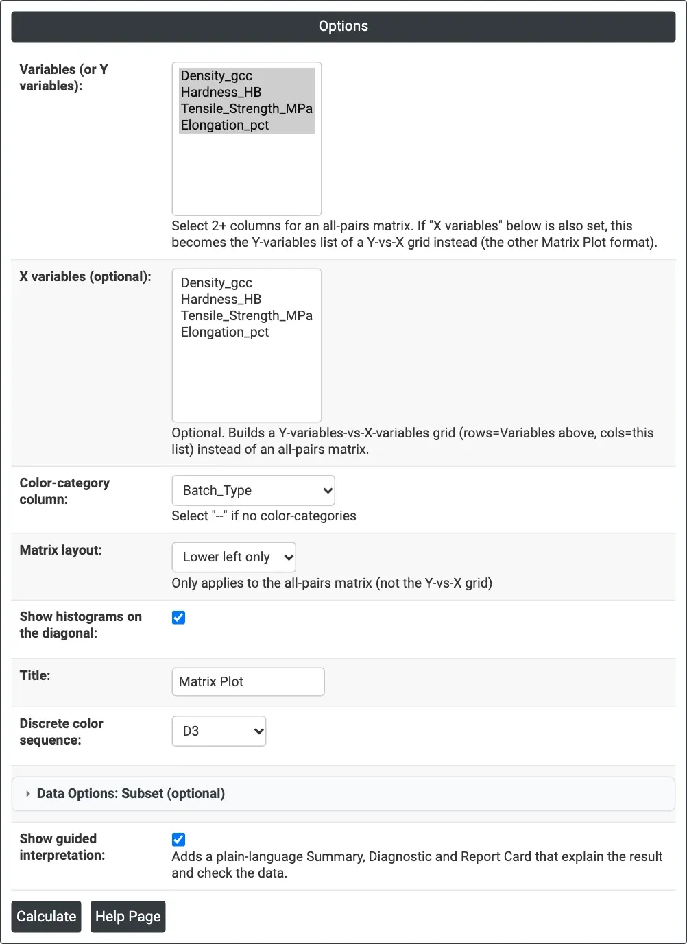
Figure 1 — Options for the example: four material properties coloured by Batch_Type, lower-left layout, histograms on the diagonal, guided interpretation on.
Output Descriptions
- Matrix Plot — the grid of scatterplots, with a histogram of each variable on the diagonal when that option is ticked, coloured by category with a legend when one is chosen; hover over a point to read its values.
- Predictive Ability Report — bar chart and table of the best model (Linear or Quadratic) and its R-sq(adj) % for each X as a predictor of the first variable (guided interpretation only).
- Diagnostic Report — what patterns to look for in each panel (guided interpretation only).
- Report Card — checks on unusual data, alternative graphs and next steps (guided interpretation only).
- PDF export via Download.
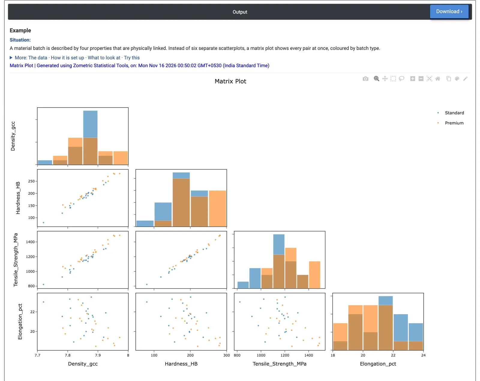
Figure 2 — Lower-left matrix of density, hardness, tensile strength and elongation for 40 batches, Standard (blue) and Premium (orange), with each property's histogram on the diagonal.
Worked Example
A metallurgist has four properties for each of 40 material batches (20 Standard, 20 Premium): density (g/cc), hardness (HB), tensile strength (MPa) and elongation (%). Instead of six separate scatterplots, the metallurgist selects all four as Variables, sets Color-category column = Batch_Type and Matrix layout = Lower left only, keeps Show histograms on the diagonal ticked and ticks Show guided interpretation.
Density, hardness and tensile strength rise together in narrow straight bands: their correlations are 0.97 to 0.99. Elongation goes the other way, more loosely: stronger batches are less ductile (correlations about −0.46 to −0.51). Premium batches sit higher in hardness (mean 212.9 against 180.1 HB) and tensile strength (1253.6 against 1126.2 MPa), while their density differs little (7.878 against 7.850 g/cc).
The Predictive Ability Report, taking density as Y, shows hardness (R-sq(adj) 96.4%) and tensile strength (93.7%) each predict density almost fully with a straight line, while elongation explains only 18.8%. For the team this means hardness, tensile strength and density carry nearly the same information: a quick hardness test can screen batches for strength, and elongation has to be measured separately because it cannot be inferred well from the others.