
Moving Average
On this page
Purpose
Moving Average smooths a time series by replacing each value with the mean of the last few periods, so that short-term noise or a repeating season fades and the underlying level or trend shows. Use it to see where a series is heading, for example monthly sales, weekly scrap or daily output, before choosing a forecasting model. Set the length to one full seasonal cycle (12 for monthly data with a yearly season) and the season cancels out. It also gives one-step-ahead fits with accuracy measures and simple flat forecasts, but for forecasting a series with a trend or a season, Double Exponential Smoothing, Winters' Method or Decomposition are better choices.
Key Capabilities
- Moving averages of any length from 2 periods upwards.
- Centred moving averages, placed in the middle of their window so they line up with the data; even lengths use the 2×L average.
- Fits (the average of the previous L periods) with MAPE, MAD and MSD accuracy measures.
- Forecasts with prediction limits at a chosen confidence level (default 95%), from the end of the series or from an earlier row to test the method on known data.
- Plot of the data, fits, moving average and forecasts; optional results table and four-in-one residual plots.
Statistical Methods
For a length L the moving average at period t is MAₜ = (yₜ + yₜ₋₁ + … + yₜ₋L₊₁) / L, the mean of the L values ending at t; the first L − 1 periods have none. With Center the moving averages ticked, each average is moved to the middle of its window: for an odd L it is the mean of the (L − 1)/2 values on each side of t; for an even L, which has no middle period, the tool uses the 2×L moving average, with weights 1/(2L) on the two end values and 1/L on the L − 1 values between them. The first and last L/2 periods (rounded down) then have no centred average. Centring only changes the moving-average column and the dotted line on the plot.
The fit for period t is always the uncentred moving average ending at period t − 1, the forecast you would have made one period earlier, and the error is yₜ minus that fit. Accuracy is computed over the periods that have a fit: MAPE = mean |error / data| × 100, MAD = mean |error| and MSD = mean error². Every forecast equals the last uncentred moving average up to the forecast origin, so the forecasts are flat. The prediction limits are forecast ± z × √MSD, where z is the standard normal quantile for the confidence level (1.96 for 95%), with the same width for every period ahead. The series needs more than L values with no gaps.
Input Fields & Options
Field | Description |
Variable (Y) | Required. The numeric series, in time order. |
MA length | Number of periods averaged. Default 3, at least 2. Use the season length (e.g. 12 for monthly data) to remove a season. |
Center the moving averages | Unticked by default. Places each average at its middle time period instead of the trailing edge of its window. |
Number of forecasts | Default 0 (none), up to 1000. |
Confidence level (%) for forecast interval | Default 95, 1 to 99.99. Active when forecasts are requested. Level of the prediction limits. |
Forecast origin (row) | Optional, active when forecasts are requested. Forecasts start after this row, using the data up to it; blank = end of the series. Must be at least the MA length. |
Results to display | Summary table (default) or Summary table and results table. |
Residual plots (four in one) | Unticked by default. Normal probability plot, residuals versus fits, histogram and residuals versus order. |
Title | Title of the output. Default Moving Average. |
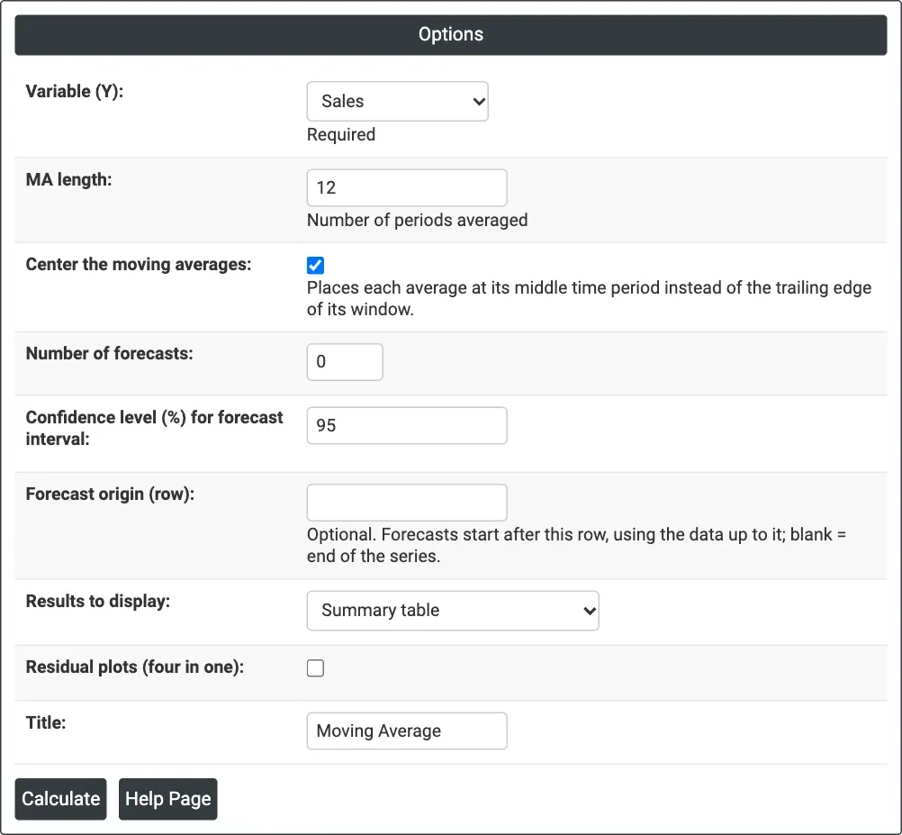
Figure 1 — Monthly Sales with a centred 12-month moving average and no forecasts.
Output Descriptions
- Moving Average (graph) — actual data, fits, the moving average (dotted) and any forecasts with their limits, with MAPE, MAD and MSD under the title.
- Method — data column, length of the series, moving average length, and Centered = Yes or the forecast origin when they apply.
- Accuracy Measures — MAPE, MAD and MSD of the fits.
- Forecasts — period, forecast, lower and upper limits, when forecasts are requested.
- Results — when chosen: Period, data, MA, Predict and Error for each period (* where there is no value).
- Residual Plots — when ticked.
- PDF export via Download.
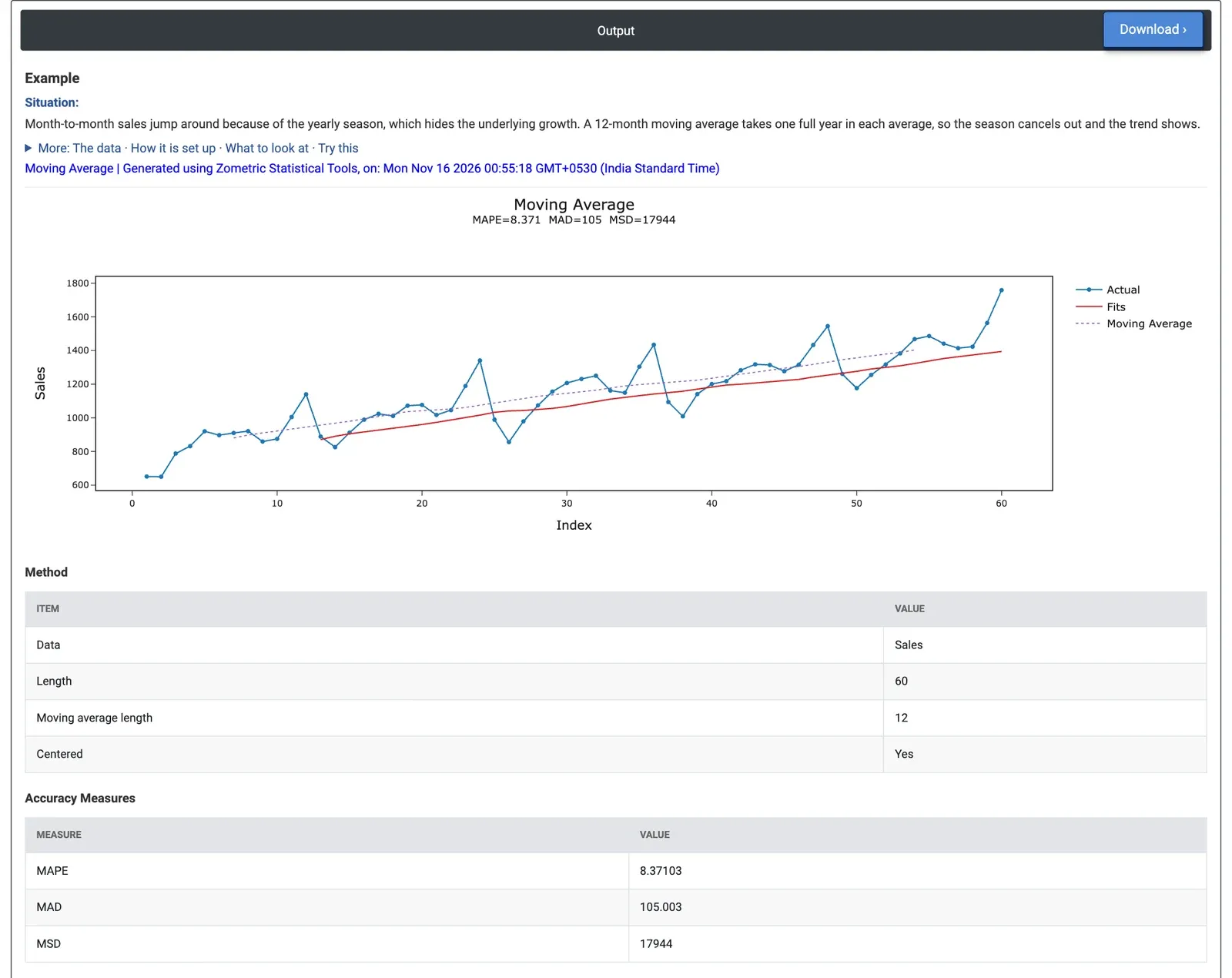
Figure 2 — The centred 12-month average climbs steadily from 881 to 1,403 with no seasonal peaks left; MAPE 8.37%, MAD 105.
Worked Example
A consumer electronics distributor has 60 months of unit sales, January 2020 to December 2024. Sales peak every December and dip every February, which hides how fast the business is growing. The sales analyst selects Variable (Y) = Sales, sets MA length = 12 so that each average covers exactly one year, and ticks Center the moving averages so that each average sits in the middle of its year.
The dotted moving-average line has no December peaks or February dips left: it climbs steadily from 881 units (July 2020, the first month with a full year around it) to 1,403 units (June 2024, the last), about 11 units a month. The first and last six months have no centred average. This is the growth the analyst wanted to see, free of the season. As a forecast of the next month the 12-month average is poor: the fits lag behind the growth and miss every peak, giving MAPE 8.37%, MAD 105 units and MSD 17,944. With MA length = 3 the line follows the season again and MAPE rises to 9.85%.
Unticking Center the moving averages and setting Number of forecasts = 12 gives 1,412.25 units for every month of 2025, the average of the 2024 sales, with 95% limits of 1,149.7 to 1,674.8. Those forecasts carry neither the growth nor the season, so the analyst uses the moving average to show the trend to management and a seasonal method such as Winters' Method or Decomposition for the 2025 plan.