
Multiple Correspondence Analysis
On this page
Purpose
Multiple Correspondence Analysis (MCA) puts every category of three or more categorical variables on one map. Categories that are often given by the same respondents or found on the same items sit close together. Use it to explore survey answers, defect records or audit findings that have several categorical fields, for example to see which customer types go with which channels and service plans, or which shifts, lines and defect types tend to occur together. For exactly two variables, use Simple Correspondence Analysis.
Key Capabilities
- Analyses three or more categorical columns at once; each category becomes a point on the map.
- Inertia table for every dimension, with percentages and cumulative percentages.
- Category table with mass, inertia, coordinates, quality, squared correlations and contributions for the number of dimensions you choose.
- Column plot of all categories on the first two dimensions, coloured by variable.
- PDF export of the results.
Statistical Methods
Rows with a missing value in any selected variable are dropped, and every value is treated as a category label. The data are turned into an indicator matrix Z with one 0/1 column per category of each variable (K columns for J variables in all). MCA is a correspondence analysis of this matrix: Z is divided by its total to give proportions P, with row masses r and column (category) masses c, and the standardised residuals S = Dr^−½ (P − r cᵀ) Dc^−½ are split by singular value decomposition. Each singular value d gives a dimension with inertia d². There are K − J dimensions, and the total inertia is always (K − J) / J, so it depends only on the number of categories, not on the data.
Category coordinates are principal coordinates, Dc^−½ V D. Mass is a category's share of the indicator matrix total, which is its relative frequency divided by J. Inert is the category's share of the total inertia. Quality is the share of the category's squared distance from the centre that the reported dimensions show (from 0 to 1); Corr is that share for one dimension, and Contr the share of a dimension's inertia that the category accounts for. Because the indicator coding spreads inertia over many dimensions, the first two dimensions in MCA usually explain a much smaller percentage than in simple correspondence analysis; the map can still be useful, but categories with low quality are not well shown.
Input Fields & Options
Field | Description |
Categorical variables | Three or more categorical columns. Hold Ctrl or Command to select several. For exactly 2 variables, use Simple Correspondence Analysis instead. |
Number of components | How many dimensions to report Quality, Corr and Contr for in the category table. Default 2; 1 to 20, limited to the number available. The plot always shows the first 2. |
Title | Title shown on the plot. Default Multiple Correspondence Analysis. |
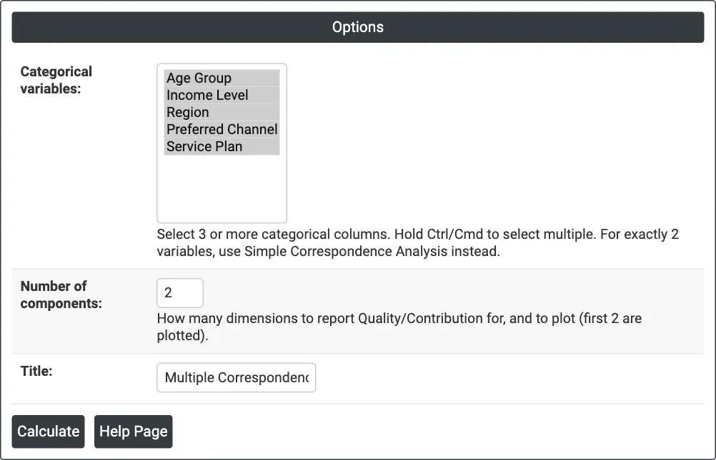
Figure 1 — Options for the example: five survey questions as categorical variables, 2 components.
Output Descriptions
- Multiple Correspondence Analysis plot — every category on Dimension 1 against Dimension 2 (percentages of inertia in the axis titles), coloured by variable. Each point is labelled with its category; the colour and the legend give the variable, and hovering shows both. Labels are placed to avoid overlapping.
- Total inertia — the total and the number of dimensions.
- Analysis of Indicator Matrix — Component (Dim1, Dim2, ...), Inertia, Percent and Cumulative Percent for every dimension.
- Column Contributions — Category, Variable, Mass, Inert, the coordinate on each reported dimension, Quality, and Corr and Contr for each reported dimension.
- PDF export via Download.
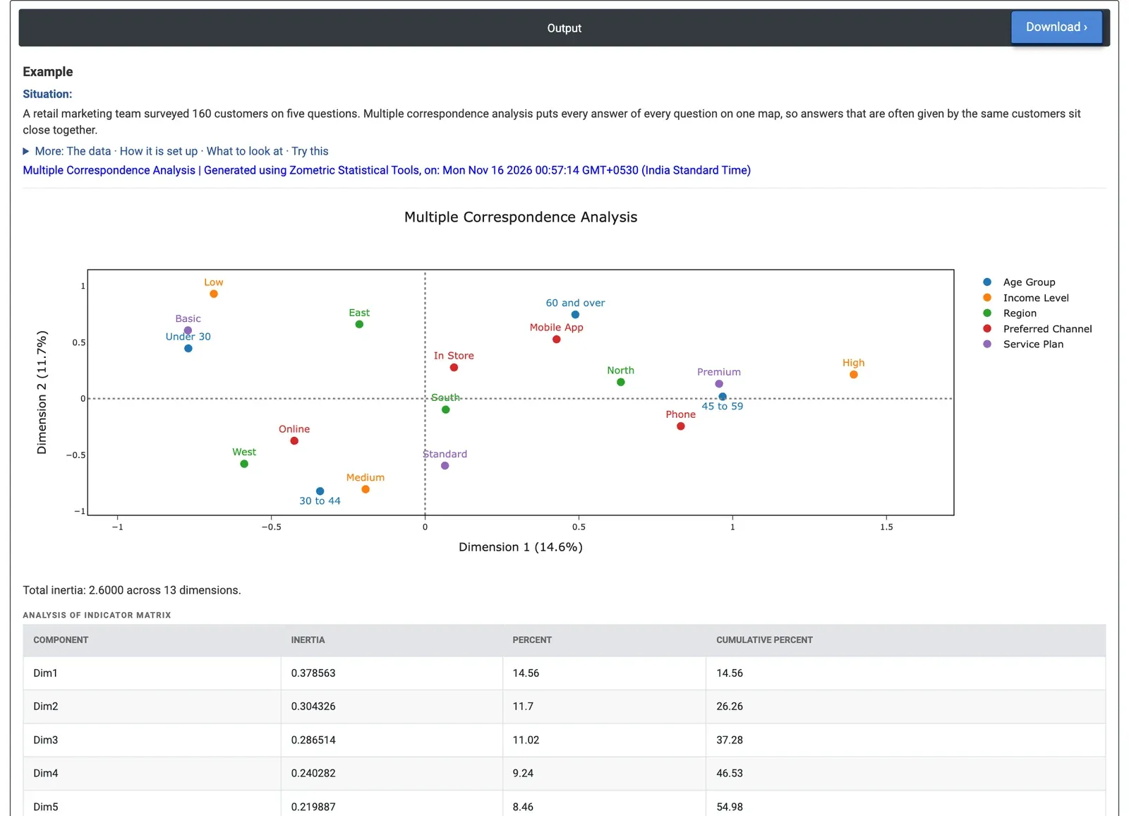
Figure 2 — Category map for five survey questions from 160 customers: Dimension 1 (14.6%) runs from low income, Basic plan and under-30s to high income, Premium plan and ages 45 to 59.
Worked Example
A retail marketing team surveyed 160 customers on five questions: age group (four groups), income level (Low, Medium, High), region (North, South, East, West), preferred channel (Online, In Store, Mobile App, Phone) and service plan (Basic, Standard, Premium). They want to see which answers go together, to plan targeted offers. They select all five columns as Categorical variables and keep Number of components = 2.
The 18 categories give 13 dimensions and a total inertia of 2.6. Dimension 1 explains 14.56% and Dimension 2 11.7%, together 26.26%: normal for MCA with this many categories, but the map should be read as a rough summary. Dimension 1 runs from Income Level: Low (−0.687), Service Plan: Basic (−0.771) and Age Group: Under 30 (−0.770) on the left to Income Level: High (1.393), Service Plan: Premium (0.956) and Age Group: 45 to 59 (0.967) on the right. Income Level: High contributes 23.1% of Dimension 1's inertia, the most of any category. On Dimension 2, Income Level: Medium (−0.804), Age Group: 30 to 44 (−0.821) and Service Plan: Standard (−0.595) sit together at the bottom.
Region: South (quality 0.0054) and Preferred Channel: In Store (0.0475) sit near the centre with very low quality: they are poorly shown on this map and do not belong to any of the groups. For the team, income level and service plan form the main pattern, with age following them, while region and channel add little. In the raw data, 60.4% of low-income customers chose Basic and 52.8% of high-income customers chose Premium. Removing Region from the analysis raises the share of the first two dimensions to 32.57%.