
Nonlinear Regression
On this page
Purpose
Nonlinear Regression fits a curve whose parameters do not enter linearly, such as an exponential approach to a limit, a saturation curve or an S-shaped growth curve, to one response and one predictor. Use it when the physics or chemistry of the process tells you the form of the curve and you want estimates of its parameters, such as a limiting value or a rate constant, with confidence intervals.
Key Capabilities
- Seven built-in expectation functions: exponential decay, exponential growth, power, 3-parameter logistic, Michaelis-Menten, Gompertz and quadratic.
- User-defined expectation function in X with parameters b1, b2, …, using + − * / ^ and exp, log, ln, log10, sqrt, abs, sin, cos, tan, arctan.
- Gauss-Newton, Levenberg-Marquardt or Trust Region Reflective fitting, with your own starting values, iteration limit and tolerance.
- Parameter estimates with standard errors and confidence intervals, and their correlation matrix.
- Fitted line plot with optional confidence and prediction bands.
- Lack-of-fit test when the predictor has repeated values.
- Optional weights column and residual plots.
Statistical Methods
The tool finds the parameter values θ that minimise the sum of squared errors SSE = Σ (yᵢ − f(xᵢ, θ))², or Σ wᵢ (yᵢ − f(xᵢ, θ))² with a weights column. Levenberg-Marquardt (default) and Trust Region Reflective use SciPy's least-squares solvers; Gauss-Newton uses step halving and reports the number of iterations. Iteration stops when the relative change in SSE and in the parameters falls below the convergence tolerance. Rows with a missing value in the response, predictor or weights are dropped.
Standard errors come from the linear approximation at the solution: Cov(θ) = MSE·(JᵀJ)⁻¹, where J is the matrix of derivatives of f with respect to the parameters and MSE = SSE / (n − p) for p parameters; S = √MSE. Confidence intervals are θ ± t(1−α/2, n−p)·SE. The confidence band for the curve uses the same approximation; the prediction band adds MSE for a single new reading. These intervals are approximate and become unreliable if the parameters are poorly determined, which shows as correlations near ±1 in the correlation matrix.
When some predictor values are repeated, the error sum of squares is split into pure error (scatter between repeats) and lack of fit, and F = MS lack-of-fit / MS pure error tests whether the chosen curve fits. Starting values matter: built-in functions start from fixed defaults (for example a = 1, b = 1 for Michaelis-Menten), with c at the median of X for the logistic and Gompertz curves; a user-defined function needs one starting value per parameter. Give values close to what you expect, or the fit may fail or find a poor local minimum.
Input Fields & Options
Field | Description |
Response (Y) / Predictor (X) | Numeric columns; must be different. Required. |
Expectation function | Exponential decay y = a·exp(−b·x) (default), Exponential growth, Power y = a·x^b, Logistic (3-param), Michaelis-Menten y = a·x/(b + x), Gompertz, Quadratic, or User-defined expectation function. |
Expectation function (user-defined) | Shown for the user-defined choice. Formula in X with parameters b1, b2, …, e.g. b1 * exp(-b2 * X). |
Weights (optional) | Column of weights for weighted least squares. |
Starting values (space-separated) | One value per parameter, in order. Optional for built-in functions (defaults used if blank), required for a user-defined one. |
Confidence level | Default 95. |
Fitting algorithm | Gauss-Newton, Levenberg-Marquardt (default) or Trust Region Reflective. |
Maximum number of iterations / Convergence tolerance | Defaults 200 and 1e-05. |
Display confidence interval on fitted curve / Display prediction interval on fitted curve | Add the bands to the fitted line plot. Off by default. |
Histogram of residuals / Normal plot of residuals / Residuals versus fits / Residuals versus order / Four in one | Residual plots; Four in one draws all four together. |
Residuals versus the variables | Plot the residuals against a chosen column. |
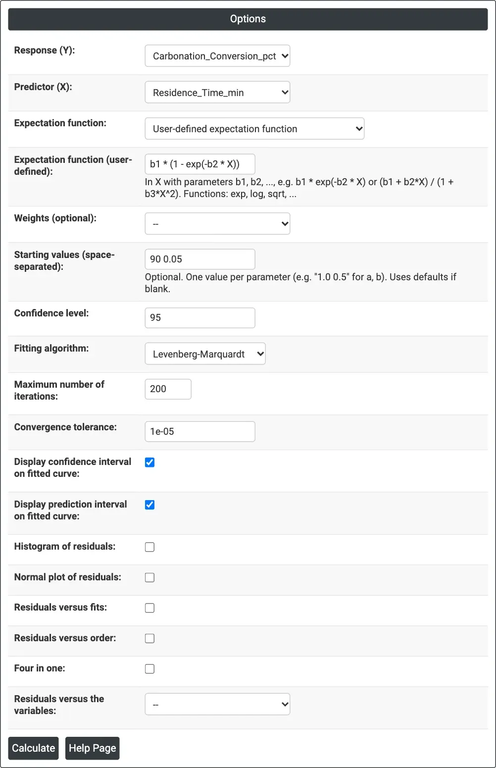
Figure 1 — Options for the carbonation example: user-defined function b1 * (1 - exp(-b2 * X)) with starting values 90 and 0.05, confidence and prediction bands ticked.
Output Descriptions
- Method — algorithm, maximum iterations, tolerance and, for Gauss-Newton, the iterations used.
- Starting Values for Parameters — the values the fit started from.
- Regression Equation — the fitted curve with the column names.
- Parameter Estimates — Estimate, SE Estimate and confidence limits for each parameter.
- Summary of Fit — Final SSE, DFE, MSE and S.
- Fitted Line Plot — data, fitted curve and optional CI and PI bands.
- Correlation Matrix for Parameter Estimates.
- Lack-of-Fit — error, lack-of-fit and pure-error rows with F and P, when the predictor has repeated values.
- Residual plots, if selected.
- PDF export via Download.
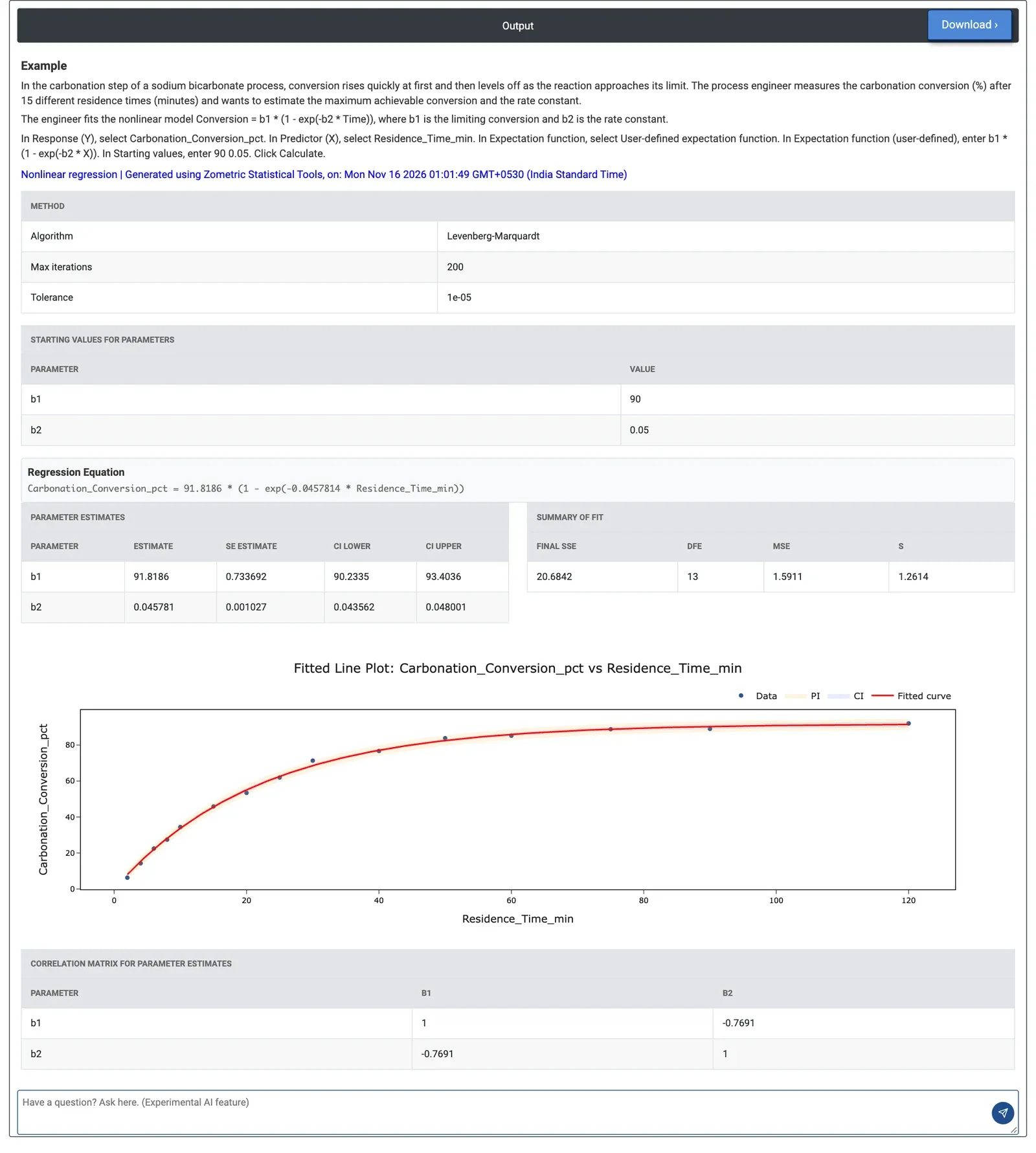
Figure 2 — Carbonation conversion against residence time: limiting conversion b1 = 91.82% and rate constant b2 = 0.0458 per minute, S = 1.26.
Worked Example
In the carbonation step of a sodium bicarbonate process, conversion rises quickly and then levels off. A process engineer measures the conversion (%) at 15 residence times from 2 to 120 minutes and wants the limiting conversion and the rate constant. The engineer enters the first-order model Conversion = b1·(1 − exp(−b2·Time)) as a user-defined function, gives starting values 90 and 0.05 and ticks both bands.
The fit converges to b1 = 91.82% (95% CI 90.23 to 93.40) and b2 = 0.0458 per minute (95% CI 0.0436 to 0.0480). S is 1.26 percentage points, small against a range of 6 to 92%, and the points sit on the curve along its whole length. The correlation between b1 and b2 is −0.77: moderate, so both parameters are well determined. Gauss-Newton gives the same estimates in 3 iterations. With no repeated residence times, no lack-of-fit test is shown.
From the fitted curve, 90% of the limiting conversion is reached at ln(10)/b2 ≈ 50 minutes and 95% at about 65 minutes; at 30 minutes the conversion is only about 69%. Residence times well beyond an hour buy little extra conversion, which helps the engineer set the tower throughput.