
Nonparametric Distribution Analysis (Right Censoring)
On this page
Purpose
Nonparametric Distribution Analysis (Right Censoring) estimates the survival curve of a product directly from life data, without assuming a Weibull, lognormal or any other distribution. It handles units that were removed or still running when observation stopped (right-censored). Use it to read off survival at given ages and the median life when no distribution fits well or you do not want to rely on one, and as a check on a parametric fit.
Key Capabilities
- Kaplan-Meier survival estimate at every observed time, with standard errors and confidence limits.
- Number at risk, number of failures and a censored flag at each time.
- Median life with a confidence interval, and a mean estimate.
- Counts of failures and right-censored units.
- Kaplan-Meier survival plot with confidence bands.
Statistical Methods
In the censoring column, rows equal to the censoring value are right-censored and every other row is a failure. The Kaplan-Meier estimate is S(t) = Π (1 − dⱼ / rⱼ) over all failure times tⱼ ≤ t, where dⱼ is the number of failures at tⱼ and rⱼ the number of units still at risk just before tⱼ. A censored unit leaves the risk set at its censoring time without causing a step, so it counts as a survivor up to that time and no further. The curve only steps down at failure times.
The standard error is S(t) times the square root of Greenwood's sum, Σ dⱼ / (rⱼ(rⱼ − dⱼ)). The confidence limits use the exponential (log-log) form of Greenwood's formula, which keeps them between 0 and 1. The median is the first time at which S(t) falls to 0.5 or below; its confidence interval runs from the first time the lower band falls to 0.5 or below to the first time the upper band does (Brookmeyer-Crowley method). The median or its limits are not estimable if the curve or band never reaches 0.5.
Mean(corrected) is the area under the Kaplan-Meier step curve from 0 to the largest observed time (the restricted mean): S = 1 up to the first time, then each estimate holds until the next listed time. If the largest observation is censored, the curve has not reached 0 and the true mean is larger, so the tool adds a warning. After the last failure the estimate stays flat: the data say nothing about failures beyond that time.
Input Fields & Options
Field | Description |
Variable | Required. Time to failure, or time to censoring for units removed or still running. |
Use censoring column | Required. Rows equal to the censoring value are right-censored; every other row is a failure. Every row needs a value. |
Censoring value | The value in the censoring column that marks a censored unit. Default 0, so 1 = failure. |
Confidence level (%) | For the survival and median confidence limits. Default 95; 50 to 99.99. |
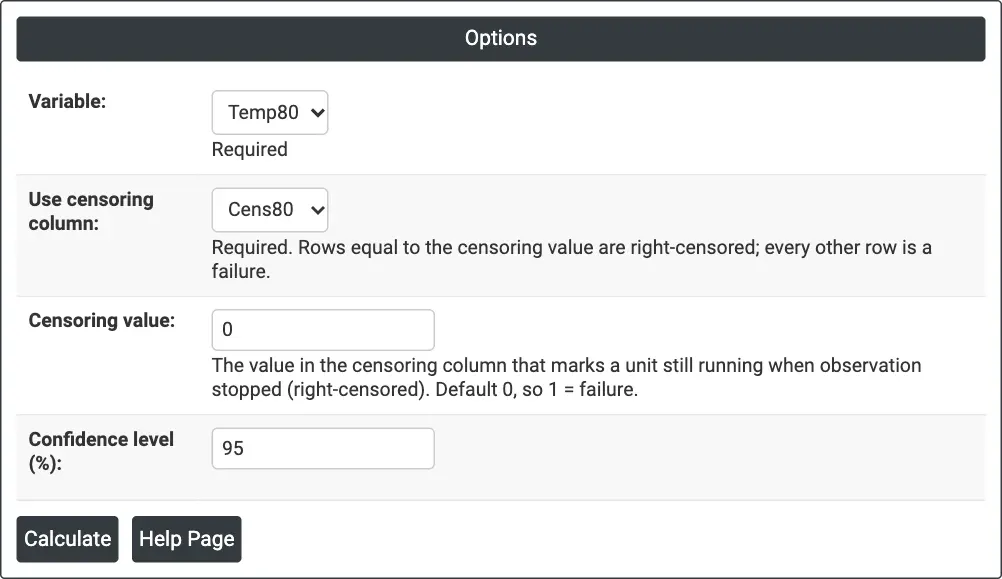
Figure 1 — Options for the example: winding test times at 80 °C (Temp80), censoring column Cens80 with censoring value 0.
Output Descriptions
- Censoring table — the number of uncensored (failure) and right-censored values.
- Characteristics — Mean(corrected) and Median with the median's confidence limits.
- Notes — for example when the mean is underestimated because the largest observation is censored, or the median is not estimable.
- Kaplan-Meier table — Time, Number at Risk, Number of Events, Censored, Survival Probability, Standard Error and confidence limits.
- Kaplan-Meier Survival Plot — the step survival curve with its confidence bands.
- PDF export via Download.
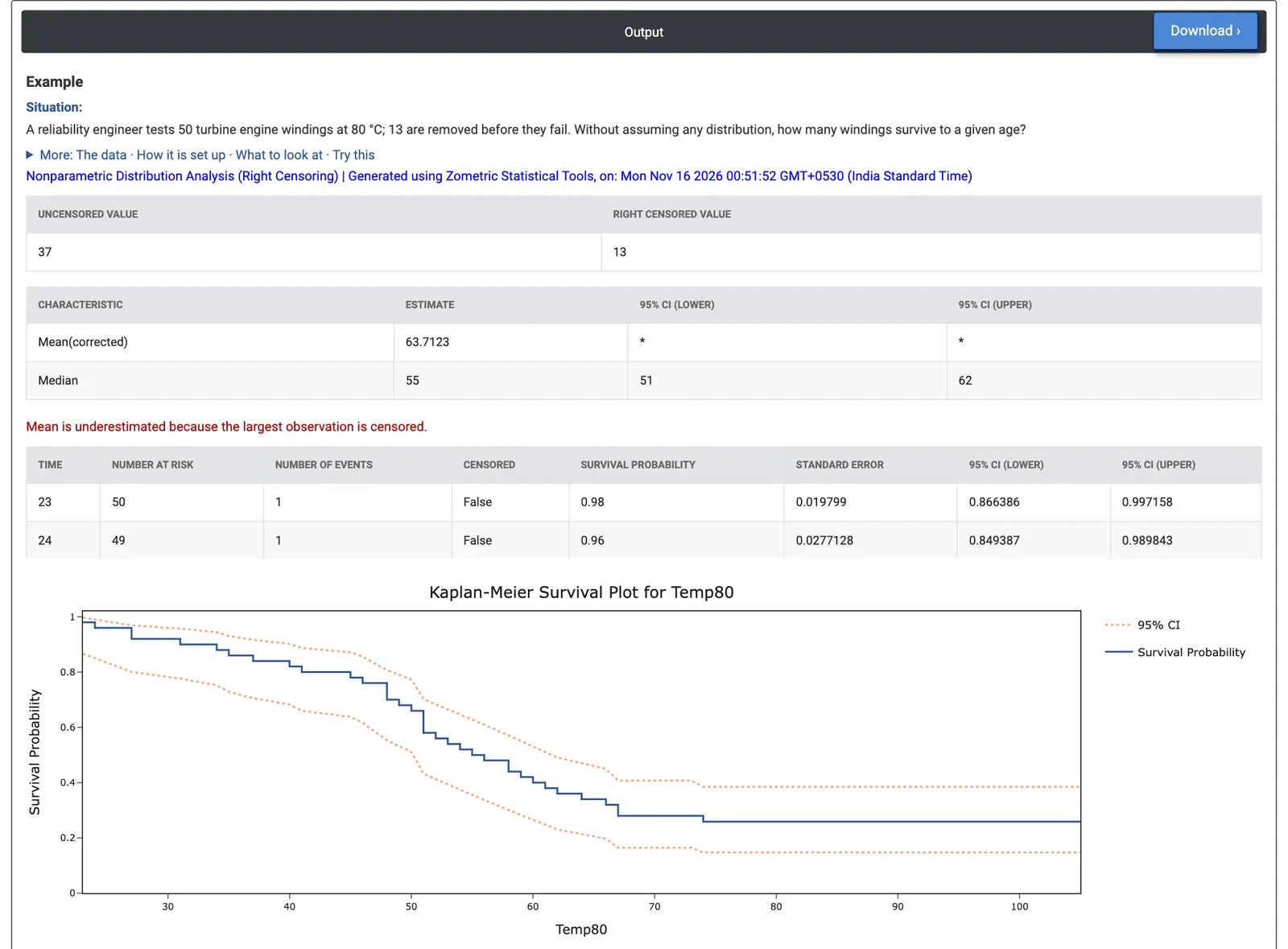
Figure 2 — Characteristics, the start of the Kaplan-Meier table and the survival plot for 50 windings: median life 55 hours (95% CI 51 to 62).
Worked Example
A reliability engineer tests 50 turbine engine windings at 80 °C. 37 fail and 13 are removed before failure. Without assuming any distribution, the engineer wants to know how many windings survive to a given age and what the median life is. They set Variable = Temp80, Use censoring column = Cens80 and Censoring value = 0, and keep 95% confidence.
The median life is 55 hours, with a 95% confidence interval of 51 to 62 hours. The estimated survival is 0.66 at 50 hours (95% CI 0.51 to 0.77) and 0.40 at 60 hours (0.27 to 0.53). The table steps down at each failure, for example from 0.66 to 0.58 at 51 hours when four windings fail together. The last failure is at 74 hours; after that every remaining winding was removed, so the curve stays at 0.258 and the data cannot say when those windings would have failed. Mean(corrected) is 63.7 hours, with the note that it is underestimated because the largest observation (105 hours) is censored.
For the engineer, the median of 55 hours is the most direct answer, with no model assumed. A Weibull fit to the same data (Distribution Overview Plot or Parametric Distribution Analysis) gives a survival of 0.66 at 50 hours, matching the Kaplan-Meier estimate, but 0.53 at 60 hours against 0.40 here, and a median of 62.6 hours. The difference shows where the Weibull model and the data part company, and which median to report depends on whether the model is trusted beyond the region where the data agree with it.