
1-Sample Poisson Rate Test
On this page
Purpose
The 1-Sample Poisson Rate Test estimates the rate at which events occur, such as defects per panel, breakdowns per month or calls per hour, and compares it with a target or historical rate. It gives the rate with a confidence interval and, if you want, a test of whether the rate differs from, or is above or below, the hypothesized value. Use it for counts of events in a fixed amount of exposure (units, area, time) where each event is independent, rather than for pass/fail results, which call for the 1 Proportion test.
Key Capabilities
- Data as a column of counts (one count per unit) or as a summary: sample size and total occurrences.
- Exact method (exact Poisson test and exact confidence interval) or normal approximation (z-test).
- Two-sided or one-sided alternatives, with a two-sided interval or a one-sided bound to match.
- Rate per unit of any length of observation, e.g. per panel, per 100 m² or per shift.
- Confidence interval only, without a test, when Perform hypothesis test is cleared.
Statistical Methods
With N units, each observed over a length t (Length of observation, default 1), the total exposure is T = N·t. If X events are counted in all, the sample rate is λ̂ = X / T. Under the null hypothesis the count X follows a Poisson distribution with mean μ₀ = λ₀·T, where λ₀ is the hypothesized rate.
Exact method: for Rate > hypothesized rate the p-value is P(X ≥ x | μ₀), for Rate < hypothesized rate it is P(X ≤ x | μ₀), and for the two-sided test the p-value adds the probability in the opposite tail beyond the count that is equally unlikely by the likelihood-ratio rule. The confidence interval is the exact (Garwood) interval from the chi-square distribution: lower = χ²(α/2; 2x) / (2T), upper = χ²(1 − α/2; 2x + 2) / (2T), with α / 2 replaced by α for a one-sided bound.
Normal approximation: z = (λ̂ − λ₀) / √(λ₀ / T), with the p-value from the standard normal distribution, and the interval λ̂ ± z·√(λ̂ / T), cut at zero. It is close to the exact method when the expected count is large. Both methods assume that events occur independently at a constant rate, so the variance of the counts equals their mean; if the counts vary much more than the mean (clusters of defects), the p-value will be too small.
Input Fields & Options
Field | Description |
Data | Summarized data (default) or Counts in a column. |
Sample | With Counts in a column: the column of counts, one per unit. Counts must be whole numbers 0 or above; blank cells are ignored. |
Sample size / Total occurrences | With Summarized data: the number of units and the total number of events counted. |
Perform hypothesis test | Ticked by default. Clear it to get only the rate and its confidence interval. |
Hypothesized rate | Required for the test. The target or historical rate per length of observation; above 0. |
Confidence level | Default 95; 75 to 100. |
Alternative hypothesis | Rate ≠ hypothesized rate (default), Rate < hypothesized rate or Rate > hypothesized rate. |
Method | Exact (default) or Normal approximation. |
Length of observation | Default 1. The amount of exposure for each unit, in the units the rate is expressed in. |
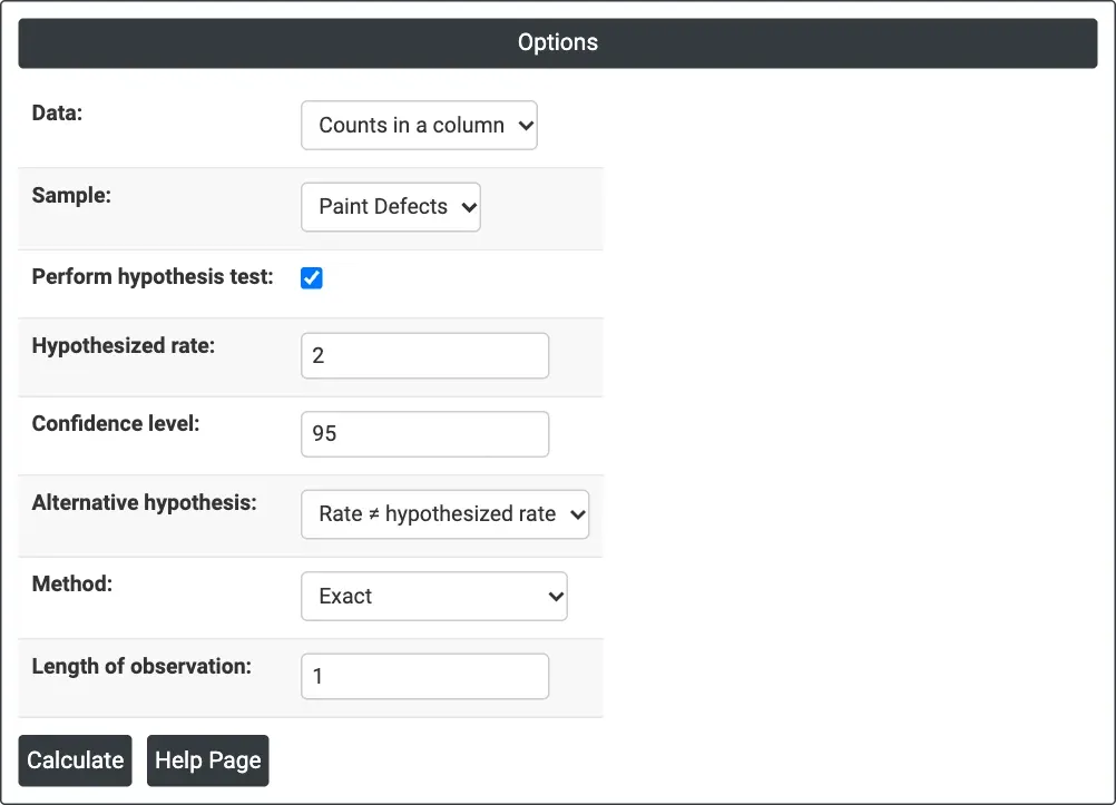
Figure 1 — Options for the example: paint defects counted on each panel, hypothesized rate 2, two-sided, exact method.
Output Descriptions
- Descriptive Statistics — N, Total Occurrences, Sample Rate and the confidence interval for λ (or a lower or upper bound for a one-sided test), with notes naming the column, the method and any length of observation other than 1.
- Test — the null and alternative hypotheses, and the P-Value (with the Z-Value for the normal approximation).
- PDF export via Download.
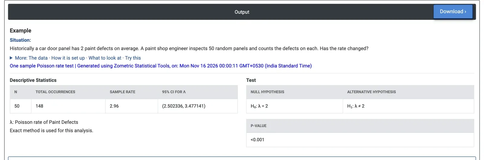
Figure 2 — 148 defects on 50 panels: a rate of 2.96 per panel, 95% CI 2.502 to 3.477, p < 0.001 against the historical rate of 2.
Worked Example
Historically a car door panel has 2 paint defects on average. A paint shop engineer inspects 50 random panels and counts the defects on each. Has the rate changed? Data = Counts in a column, Sample = Paint Defects, Hypothesized rate = 2, Confidence level = 95, Alternative hypothesis = Rate ≠ hypothesized rate, Method = Exact, Length of observation = 1.
The 50 panels have 148 defects in all, a sample rate of 2.96 defects per panel. The 95% confidence interval for λ is 2.502 to 3.477: the whole interval is above 2. The exact p-value is below 0.001, so the defect rate has changed; it is about half as high again as before. The counts look Poisson: their variance (2.37) is close to their mean, so there is no sign of defects coming in clusters that would make the test too optimistic.
The normal approximation gives the same conclusion (z = 4.8, p < 0.001, interval 2.483 to 3.437). If the question is only whether the rate has risen, Rate > hypothesized rate gives a 95% lower bound of 2.571 defects per panel: the defect rate is at least about 29% above the historical level, and the engineer should look for what changed in the paint process. The same result is obtained with Data = Summarized data, Sample size = 50 and Total occurrences = 148.