
Pairwise Averages / Differences / Slopes
On this page
Purpose
Pairwise Averages / Differences / Slopes lists every pairwise combination of your data and summarises it with a robust, distribution-free estimate. Pairwise averages give the Hodges-Lehmann estimate of a sample's centre; pairwise differences give the Hodges-Lehmann estimate of the shift between two independent samples; pairwise slopes give the Theil-Sen (Sen's slope) estimate of a trend. Use them when the data are skewed or contain outliers and you do not want a few extreme values to pull a mean or a least-squares slope.
Key Capabilities
- Three tools in one, chosen with Type: pairwise averages (one sample), pairwise differences (two independent samples) and pairwise slopes (paired X and Y).
- Hodges-Lehmann estimate of the median with a confidence interval from the Wilcoxon signed-rank test.
- Hodges-Lehmann estimate of the shift between two samples with an approximate confidence interval from the Mann-Whitney distribution.
- Theil-Sen slope: the median of all pairwise slopes.
- Table of the pairwise values (first 200 shown) and a histogram of all of them.
- Data Options: subset the rows before the analysis.
Statistical Methods
Pairwise averages: for n observations the tool forms all n(n + 1)/2 Walsh averages (xᵢ + xⱼ)/2 with i ≤ j, including each value with itself. Their median is the Hodges-Lehmann estimate of the population median (the centre of a symmetric distribution). The confidence interval contains every Walsh average that the two-sided Wilcoxon signed-rank test, used as a test of the median, does not reject at α = 1 − confidence level (exact test up to 50 observations, normal approximation above).
Pairwise differences: for samples of sizes n₁ and n₂ the tool forms all n₁·n₂ differences xᵢ − yⱼ; their median is the Hodges-Lehmann estimate of the shift between the two populations. The approximate confidence interval runs from the (k+1)-th smallest to the (k+1)-th largest difference, with k = floor(n₁n₂/2 − z·√(n₁n₂(n₁ + n₂ + 1)/12)), the normal approximation to the Mann-Whitney statistic. Missing values are dropped from each sample separately.
Pairwise slopes: for n paired (x, y) observations the tool forms the slope (yⱼ − yᵢ)/(xⱼ − xᵢ) for every pair with different x values; pairs with tied x are skipped. The median of these slopes is the Theil-Sen estimate, which is not affected by up to about 29% of wild points. No confidence interval is given for the slope. All three estimates assume independent observations; pairwise averages also assume a roughly symmetric distribution.
Input Fields & Options
Field | Description |
Type | Pairwise Averages (one sample: Walsh averages / Hodges-Lehmann estimator, default), Pairwise Differences (two independent samples: Hodges-Lehmann shift estimator) or Pairwise Slopes (paired X/Y: Theil-Sen / Sen's slope estimator). |
Variable | Numeric column. Required for Pairwise Averages. |
First sample / Second sample | Numeric columns. Required for Pairwise Differences; the differences are first − second. |
X variable / Y variable | Numeric columns of paired values. Required for Pairwise Slopes. |
Confidence level | Default 95, from 75 to 100. Used for Pairwise Averages and Pairwise Differences only. |
Data Options: Subset (optional) | Exclude matching rows (default) or Include only matching rows, by row numbers and/or a condition. |
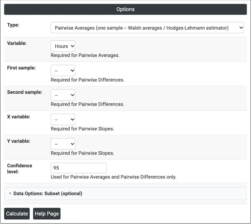
Figure 1 — Options for the bulb life example: Pairwise Averages of Hours at 95% confidence.
Output Descriptions
- Summary table — the column(s) used, N (or N1 and N2), the number of pairwise values, the estimate (Hodges-Lehmann median, Hodges-Lehmann shift or Theil-Sen slope) and, for averages and differences, the confidence interval.
- Table of pairwise values — sorted, first 200 rows.
- Histogram of all the pairwise values.
- PDF export via Download.
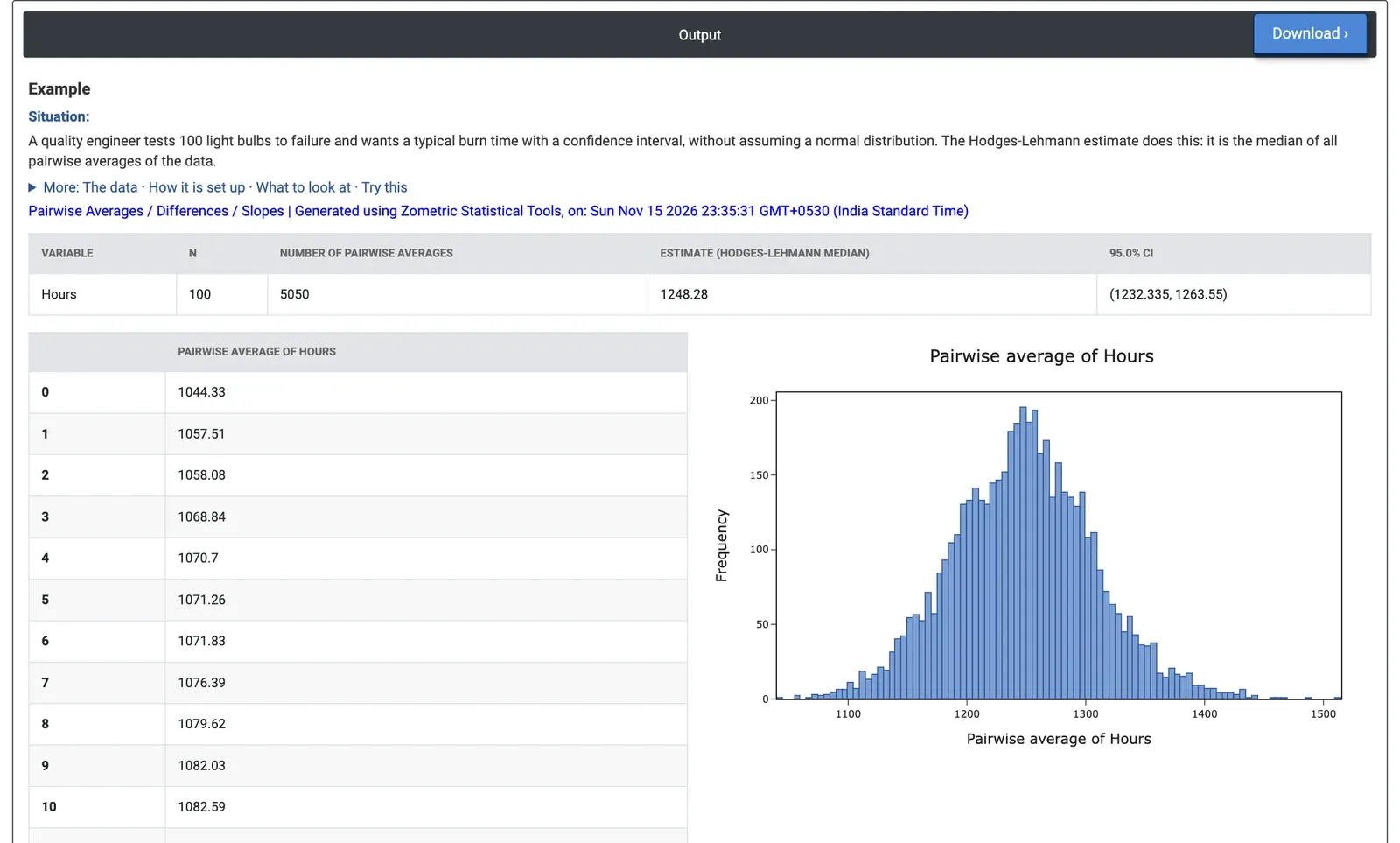
Figure 2 — Pairwise averages of the burn times: 5050 Walsh averages, Hodges-Lehmann estimate 1248.28 hours, 95% CI 1232.335 to 1263.55 hours.
Worked Example
A quality engineer tests 100 light bulbs to failure (Hours, 1044 to 1510 hours) and wants a typical burn time with a confidence interval, without assuming a normal distribution. The engineer chooses Pairwise Averages, selects Hours as the variable and keeps 95% confidence.
The tool forms 100 × 101 / 2 = 5050 pairwise averages. Their median, the Hodges-Lehmann estimate of the typical burn time, is 1248.28 hours, with a 95% confidence interval of 1232.335 to 1263.55 hours. The histogram of the pairwise averages is single-peaked and nearly symmetric around that value.
For comparison, the ordinary mean of the data is 1248.00 hours and the t-based 95% interval is about 1231.3 to 1264.7 hours: with these fairly symmetric data the robust and the classical answers agree, which gives the engineer confidence in the figure. With skewed data or a few very early failures, the Hodges-Lehmann estimate would move much less than the mean. To compare two bulb designs, the engineer would choose Pairwise Differences and read the Hodges-Lehmann shift and its interval.