
Parametric Distribution Analysis (Arbitrary Censoring)
On this page
Purpose
Parametric Distribution Analysis (Arbitrary Censoring) fits a life distribution to failure data in which exact failure times are often unknown: units found failed at an inspection (interval-censored), units already failed at the first check (left-censored), and units still working when last seen (right-censored), mixed with any exact failures. It reports the distribution's parameters, mean, median, quartiles and a full table of percentiles. Use it to estimate B10 life, warranty-period failure fractions or median life from inspection or audit records. With a Weibull distribution and a known shape, it can also run a Weibayes analysis.
Key Capabilities
- Data entered as a Start column and an End column; the pattern of blank and filled cells sets the type of censoring on each row.
- Six distributions: Weibull, Lognormal, Exponential, Normal, Logistic and Loglogistic.
- Maximum likelihood estimates with standard errors and confidence intervals at the confidence level you set.
- Mean, standard deviation, median, quartiles and the time by which 1% to 99% of units fail.
- Weibayes option for Weibull: fix the shape from past knowledge and estimate only the scale, with confidence bounds and reliability at chosen times.
- Probability plot with the fitted line and confidence bounds.
Statistical Methods
Each row is read from its Start and End values: Start = End is an exact failure; Start < End is an interval-censored failure between the two times; End blank is right-censored at Start; Start blank is left-censored at End. The censoring table counts each type. The distribution is fitted by maximum likelihood: an exact failure contributes the density f(t), a right-censored unit 1 − F(Start), a left-censored unit F(End) and an interval-censored unit F(End) − F(Start). Standard errors come from the inverse of the Hessian of the log-likelihood at the estimate, and the confidence intervals use z from the normal distribution for the Confidence level (1.96 for 95%). As in Minitab, a parameter that must be positive (a scale, shape, sigma or rate) gets its interval on the log scale, from estimate / exp(z × SE / estimate) to estimate × exp(z × SE / estimate), which keeps it positive and makes it asymmetric; a location parameter Mu gets estimate ± z × SE. The probability plot adds two-sided confidence bounds for the percentiles, as Minitab draws them: for each percent p, the percentile t_p and its variance by the delta method from the same covariance matrix, with the interval formed on ln(t_p) for Weibull, Lognormal, Exponential and Loglogistic and on t_p for Normal and Logistic.
The characteristics and percentiles are computed from the fitted distribution: the p-th percentile is the time by which p% of units are expected to fail, so the 10th percentile is the B10 life. The goodness-of-fit table gives the log-likelihood, which can be compared between distributions with the same number of parameters (higher is better). The Anderson-Darling statistic is added only when there are at least two exact failures. The probability plot shows the Turnbull nonparametric estimate of the cumulative probability of failure, on axes that make the chosen distribution a straight line, with the fitted line.
When a Known shape (Weibayes) is entered for a Weibull fit, the shape is fixed and only the scale is estimated by maximum likelihood, with likelihood-ratio confidence bounds when the data include left- or interval-censored rows, and chi-square (time-terminated) bounds when they are only exact and right-censored. This works even with very few or no failures; with no failures the tool also reports the classic Weibayes estimate, which assumes one failure is about to happen. The Confidence interval and reliability-time fields are used only in this case; the Confidence level is used in both cases.
Input Fields & Options
Field | Description |
Start column | Required. Last known good time, or the exact failure time. Leave Start blank on a row to mark it left-censored. |
End column | Required. First known failed time, or the exact failure time. Leave End blank on a row to mark it right-censored. Start = End means an exact failure; Start < End means interval-censored. Must differ from the Start column. |
Assumed distribution | Required. Weibull, Lognormal, Exponential, Normal, Logistic or Loglogistic. |
Known shape (Weibayes) | Shown for Weibull. Optional: fixes the Weibull shape at this value and estimates only the scale. Leave blank to estimate both. |
Confidence level | Default 95; 50 to 99.99. Sets the parameter confidence intervals and the probability-plot bounds, and the Weibayes bounds when a known shape is entered. |
Confidence interval | Weibayes only. Lower bound (default), Two-sided or Upper bound. |
Estimate reliability at times | Weibayes only. Optional, space-separated times, e.g. 500 1000, at which to report reliability with its bound. |
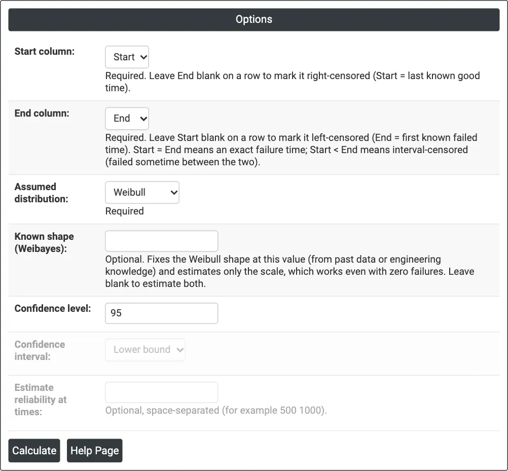
Figure 1 — Options for the example: inspection data in Start and End columns, Weibull distribution with the shape estimated.
Output Descriptions
- Censoring table — the number of uncensored, left-censored, interval-censored and right-censored values, and the estimation method.
- Parameter estimates — each parameter with its estimate, standard error and confidence limits at the chosen level (for Weibayes: the known shape and the scale with its bound).
- Goodness of fit — log-likelihood, and Anderson-Darling when there are at least two exact failures.
- Characteristics — Mean, Standard deviation, Median, First quartile (Q1), Third quartile (Q3) and Interquartile range (IQR).
- Percentiles — the time by which 1%, 2%, ..., 10%, 20%, ..., 90%, 91%, ..., 99% of units fail.
- Reliability — Weibayes only, at the times entered.
- Probability plot — the Turnbull estimates, the fitted line and its confidence bounds (dotted).
- PDF export via Download.
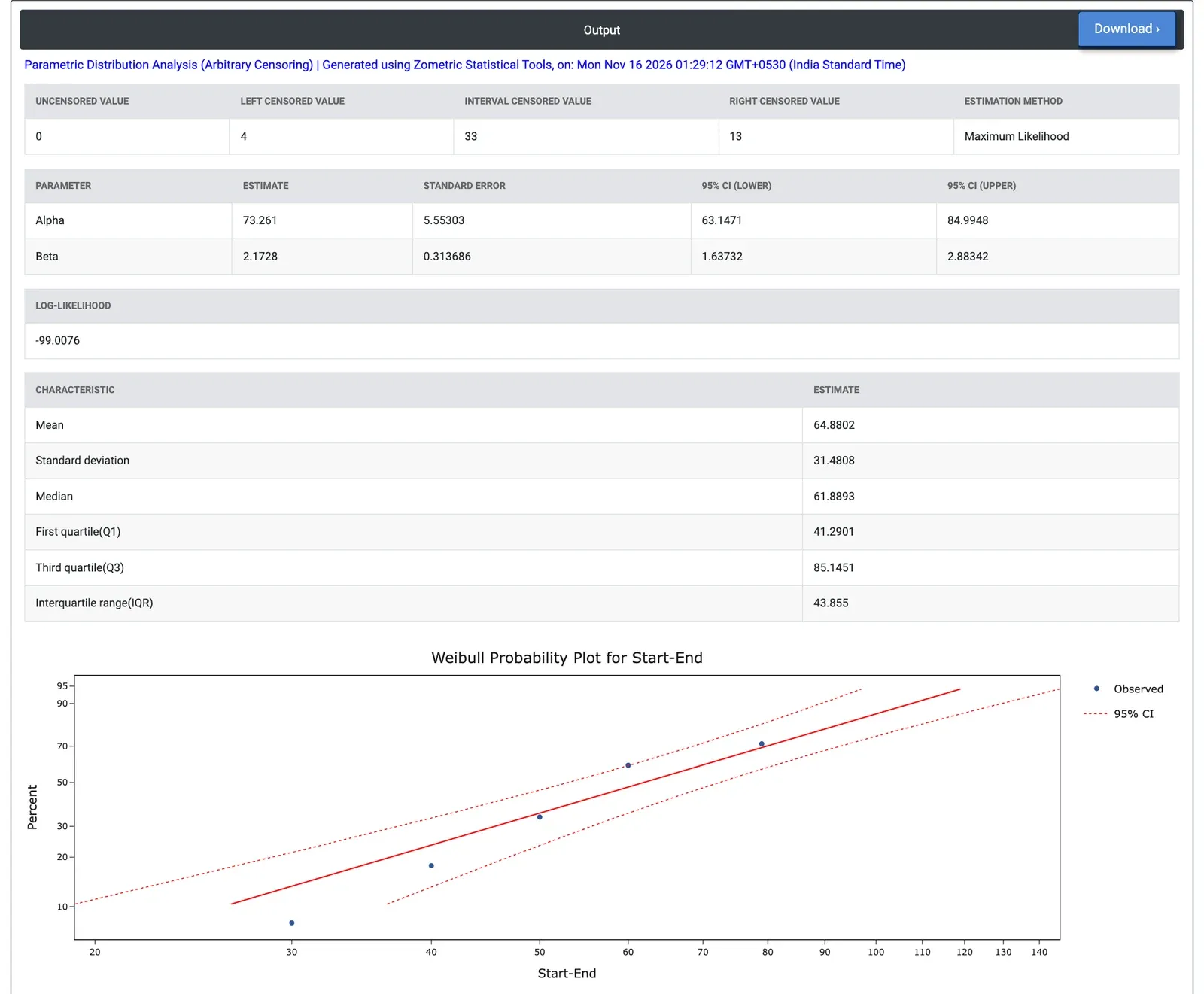
Figure 2 — Weibull fit to 50 windings checked every 10 hours: scale 73.3 h, shape 2.17, median 61.9 h, with the probability plot and its 95% bounds (the percentile table is not shown).
Worked Example
Turbine engine windings are tested at 80 °C but checked only at inspections every 10 hours from 30 hours. This example uses the 50 windings of the right-censoring examples recorded that way: 4 are found failed at the first inspection (left-censored, End = 30), 33 are found failed at a later inspection (interval-censored, for example Start = 50, End = 60), and 13 are removed before failure (right-censored, End blank). The engineer selects Start and End as the Start and End columns and Assumed distribution = Weibull, leaving Known shape blank.
The fitted Weibull has scale Alpha = 73.26 hours (95% CI 63.15 to 84.99) and shape Beta = 2.173 (95% CI 1.637 to 2.883), the same as Minitab gives for these data. Because the whole interval for the shape lies above 1, the failure rate rises with age: wear-out. The mean life is 64.88 hours, the median 61.89 hours and the quartiles 41.29 and 85.15 hours. From the percentile table, 10% of windings are expected to fail by 26.0 hours (the B10 life) and 90% by 107.5 hours. These are close to the fit from exact failure times (scale 73.34 hours, shape 2.318), so the 10-hour inspections cost little precision here. At Confidence level 90 the intervals narrow to 64.67 to 82.99 hours for the scale and 1.714 to 2.755 for the shape.
The log-likelihood is −99.01. Lognormal (−95.93) and Loglogistic (−95.51) give higher log-likelihoods with the same number of parameters, so they fit these grouped data somewhat better; their medians are 59.6 and 58.5 hours, and their B10 lives are 31.1 and 30.4 hours against 26.0 hours for Weibull. Weibull gives the more cautious early-life figure, so check the lower percentiles with more than one distribution before committing to a warranty figure. With Known shape (Weibayes) = 2, the scale is 73.37 hours with a 95% lower bound of 64.45 hours, and entering 40 under Estimate reliability at times gives a reliability of 0.743 at 40 hours with a 95% lower bound of 0.680.